cover

Snedecor's F distribution and F-test

June 19, 2021 13 min read

Here I discuss, how to derive F distribution as a random variable, which is a ratio of two independent chi-square disributions. I'll also briefly discuss F-test and ANOVA here.

In my previous posts I’ve described Chi-square distribution (as a special case of Gamma distribution) and Pearson’s Chi-square test, from which many other distributions and tests are derived in the field of statistics.

In this post I am going to derive the distribution function of a Snedecor’s F distribution. It is essentially a ratio between two independent Chi-square-distributed variables with nn and mm degrees of freedom respectively ξ=χn2χm2\xi = \frac{\chi_n^2}{\chi_m^2}.

In order to infer its probability density function/cumulative distribution function from the ratio, I’ll have to discuss non-trivial technicalities about measure theory etc. first.

Conditional probabilities of multi-dimensional continuous variables

Suppose that we need to calculate the probability density function of a random variable ξ\xi, which is a multiple of 2 independent random variables, η\eta and ψ\psi.

First, let us recall the definition of independent random variables in a continuous case: fη,ψ(x,y)=fη(x)fψ(y)f_{\eta, \psi}(x,y) = f_\eta(x) \cdot f_\psi(y). Basically, joint probability density function is a multiplication of individual probability density functions.

Thus, cumulative distribution function Fη,ψ(x,y)=t=xs=yfη(t)fψ(s)dtdsF_{\eta,\psi}(x, y) = \int \limits_{t=-\infty}^{x} \int \limits_{s=-\infty}^{y} f_{\eta}(t) f_{\psi}(s) dt ds.

Now, we need to calculate the cumulative distribution function of a multiple of 2 random variables. The logic is similar to convolutions in case of a sum of variables: if the product ηψ=x\eta \psi = x, we allow η\eta to take an arbitrary value of tt, and ψ\psi should take value of xt\frac{x}{t} then.

We will be integrating fη(t)fψ(s)f_{\eta}(t) f_{\psi}(s) in a space, where s=xts=\frac{x}{t}, we have to multiply the integrand by Jacobian determinant dsdx=1t\left|\frac{ds}{dx}\right| = \frac{1}{t}.

Thus, probability density function of F distribution is fχn2χm2(x)=t=0fχn2(t)f1χm2(xt)1tdtf_{\frac{\chi_n^2}{\chi_m^2}}(x) = \int \limits_{t=0}^{\infty} f_{\chi^2_n}(t) f_{\frac{1}{\chi^2_m}}(\frac{x}{t}) \frac{1}{t} dt.

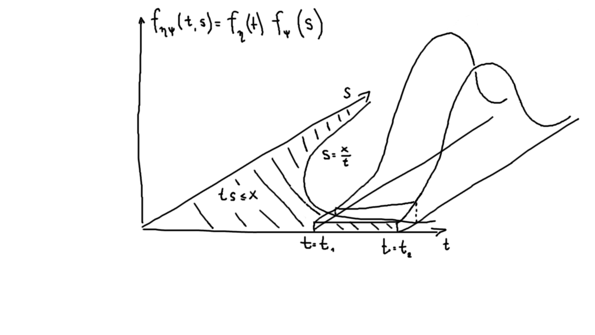
Similarly, cumulative distribution function Fηψ(x)=t=0s=0x/tfη(t)fψ(s)dtds=t=0Fψ(xt)fη(t)dt=t=0p(ψxt)dFη(t)=t=0p(ψxt)p(tη<t+dt)F_{\eta\psi}(x) = \int \limits_{t=0}^{\infty} \int \limits_{s=0}^{x/t}f_\eta(t) f_\psi(s) dt ds = \int \limits_{t=0}^{\infty}F_\psi(\frac{x}{t})f_\eta(t)dt = \int \limits_{t=0}^{\infty}p(\psi \leq \frac{x}{t})dF_\eta(t) = \int \limits_{t=0}^{\infty}p(\psi \leq \frac{x}{t}) p(t \leq \eta < t+dt) (note that multiplication of integrand by Jacobian is not required here, as this is a proper 2D integral).

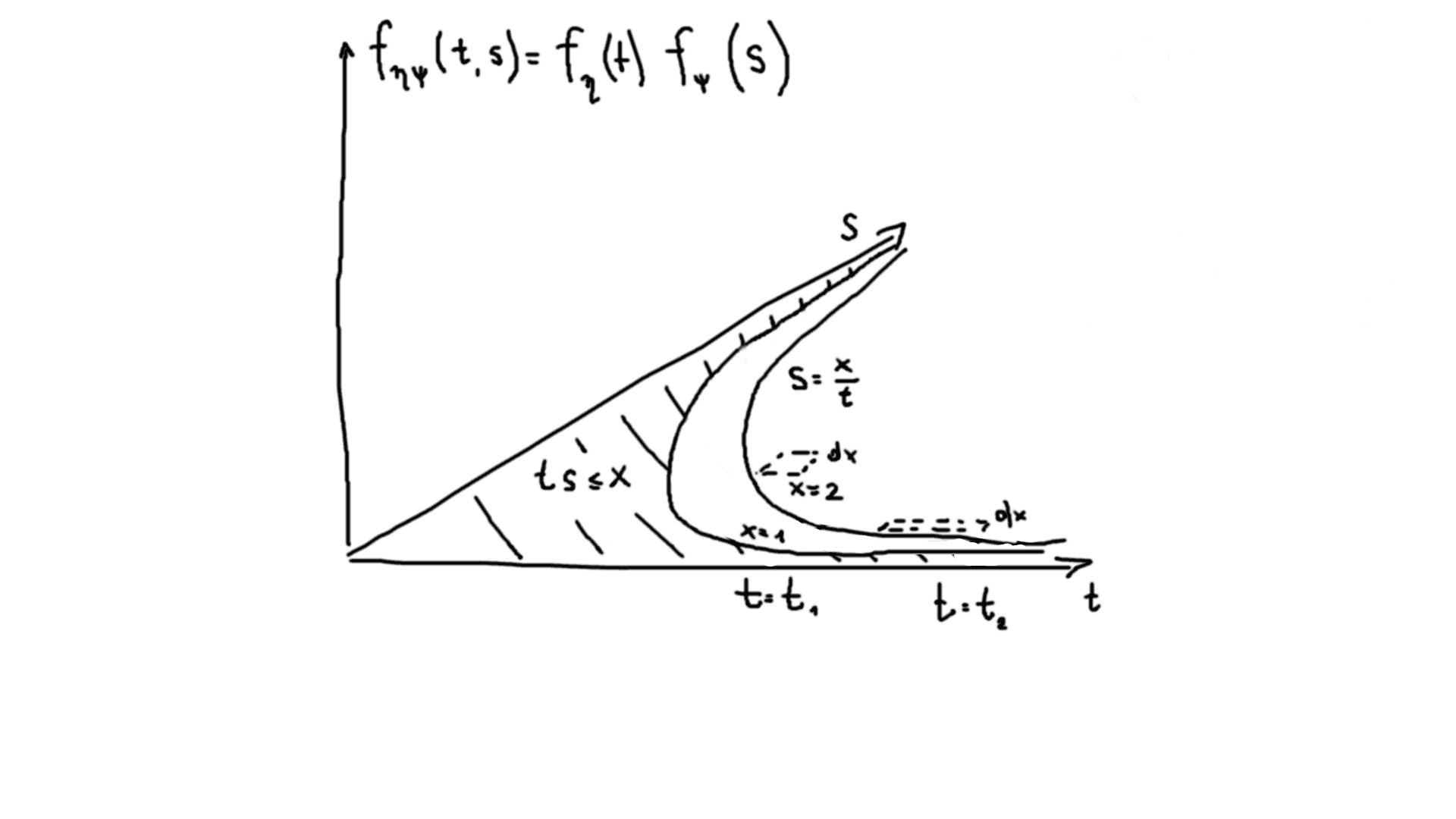
Graphically, it represents the integral of 2-dimensional probability density function over the area, delimited by s=xts=\frac{x}{t} curve:

2-dimensional pdf

Off-topic consistency considerations

Please, skip this section, it is a memento for myself, the product of my attempts to reason about how this integration works.

Suppose, we want to get c.d.f. from p.d.f.: Fηψ(x)=x=+fηψ(x)dxF_{\eta\psi}(x) = \int \limits_{x=-\infty}^{+\infty}f_{\eta\psi}(x)dx. How to interpret it? x=tsx=ts is an area, so dxdx is a unit rectangle; fηψ(x)f_{\eta\psi}(x) is an integral of fψ(s)fη(t)f_\psi(s)f_\eta(t) over the length of each hyperbola, corresponding to a single xx value. When we integrate over the length of each hyperbola, as we approach infinity with s, t approaches zero, so the area of x stays the same.

2-dimensional pdf integration

A consistency consideration: we can infer p.d.f. from inequalities directly and see that integration is consistent:

fηψ(x)dx=dFηψ(x)=p(xηψ<x+dx)=t=dFψ(xt)dFη(t)=t=dFψ(xt)fη(t)dt=t=p(xtψ<xt+dxt)p(tη<t+dt)=t=p(xηψ<(t+dt)(xt+dxt))=f_{\eta\psi}(x)dx = dF_{\eta\psi}(x) = p(x \leq \eta\psi < x+dx) = \int \limits_{t=-\infty}^{\infty} dF_\psi(\frac{x}{t}) dF_\eta(t) = \int \limits_{t=-\infty}^{\infty} dF_\psi(\frac{x}{t}) f_\eta(t)dt = \int \limits_{t=-\infty}^{\infty} p(\frac{x}{t} \leq \psi < \frac{x}{t} + d\frac{x}{t}) p(t \leq \eta < t+dt) = \int \limits_{t=-\infty}^{\infty} p(x \leq \eta \psi < (t+dt)(\frac{x}{t} +d \frac{x}{t}) ) =

=t=p(xηψ<(txt+xtdt+t(xdtt2+dxt)+dtdxt))=t=p(xηψ<x+xtdtxtdt+dx)=t=dFηψ(x)=dFηψ(x) = \int \limits_{t=-\infty}^{\infty} p(x \leq \eta \psi < (t\frac{x}{t} + \frac{x}{t}dt + t\cdot(-\frac{xdt}{t^2} + \frac{dx}{t}) + \cancel{dt \cdot d\frac{x}{t}})) = \int \limits_{t=-\infty}^{\infty} p(x \leq \eta\psi < x + \cancel{\frac{x}{t}dt} - \cancel{\frac{x}{t}dt} + dx) = \int \limits_{t=-\infty}^{\infty} dF_{\eta\psi}(x) = dF_{\eta\psi}(x).

Snedecor’s F distribution derivation

We want to calculate the probability density function of F distribution as a multiple of 2 distributions, chi-square and inverse chi-square. But we need to invert χm2\chi_m^2 first to do so. We’ll have to derive the probability density function of inverse chi-square distribution.

Inverse chi-square distribution

Recall the probability density function of chi-square distribution: fχn2=xn21ex/22n2Γ(n/2)f_{\chi_n^2} = \frac{x^{\frac{n}{2}-1} e^{-x/2}}{2^{\frac{n}{2}}\Gamma(n/2)}.

By inverse distribution formula: Fχ2(x)=p(χ2x)=p(1χ21x)=1p(1χ21x)=1F1χ2(1x)F_{\chi^2}(x) = p(\chi^2 \leq x) = p(\frac{1}{\chi^2} \geq \frac{1}{x}) = 1 - p(\frac{1}{\chi^2} \leq \frac{1}{x}) = 1 - F_{\frac{1}{\chi^2}}(\frac{1}{x}).

Thus, fχ2(x)=(1F1χ2(1x))x=1x2f1χ2(1x)f_{\chi^2}(x) = \frac{\partial (1-F_{\frac{1}{\chi^2}}(\frac{1}{x}))}{\partial x} = \frac{1}{x^2} f_{\frac{1}{\chi^2}}(\frac{1}{x}). Now, if x=1yx=\frac{1}{y}, fχ2(1y)=y2f1χ2(y)f_{\chi^2}(\frac{1}{y}) = y^2f_{\frac{1}{\chi^2}}(y) and f1χ2(y)=1y2fχ2(1y)f_{\frac{1}{\chi^2}}(y) = \frac{1}{y^2}f_{\chi^2}(\frac{1}{y}).

As a result, p.d.f. of inverse chi-square f1χ2(x)=1x21xn21e12x2n2Γ(n2)=1xn2+1e12x2n2Γ(n2)f_{\frac{1}{\chi^2}}(x) = \frac{1}{x^2} \cdot \frac{\frac{1}{x}^{\frac{n}{2}-1} \cdot e^{-\frac{1}{2x}} }{2^{\frac{n}{2}} \Gamma(\frac{n}{2})} = \frac{\frac{1}{x}^{\frac{n}{2}+1} \cdot e^{-\frac{1}{2x}} }{2^{\frac{n}{2}} \Gamma(\frac{n}{2})}.

F-distribution

Now, let us substitute the p.d.f. of chi-square and inverse chi-square distributions into F-distribution probability density function:

fχn2χm2(x)=t=0fχn2(t)f1χm2(xt)1tdsdxdt=t=0tn/21et/22n/2Γ(n/2)txm/2+1et2x2m/2Γ(m/2)1tdt=f_{\frac{\chi_n^2}{\chi_m^2}}(x) = \int \limits_{t=0}^{\infty} f_{\chi^2_n}(t) f_{\frac{1}{\chi^2_m}}(\frac{x}{t}) \underbrace {\frac{1}{t}}_{\left| \frac{ds}{dx} \right|} dt = \int \limits_{t=0}^{\infty} \frac{t^{n/2-1}e^{-t/2}}{2^{n/2}\Gamma(n/2)} \frac{{\frac{t}{x}}^{m/2+1}e^{-\frac{t}{2x}}}{2^{m/2}\Gamma(m/2)} \frac{1}{t} dt =

=1Γ(n/2)Γ(m/2)2m+n2xm/2+1t=0tn+m21e(t+tx)/2dt=1Γ(n/2)Γ(m/2)2m+n2xm/2+1t=0tn+m21et2(1+1x)dt = \frac{1}{\Gamma(n/2)\Gamma(m/2) 2^{\frac{m+n}{2}} x^{m/2+1}} \int \limits_{t=0}^{\infty}t^{\frac{n+m}{2}-1}e^{-(t+\frac{t}{x})/2}dt = \frac{1}{\Gamma(n/2)\Gamma(m/2) 2^{\frac{m+n}{2}} x^{m/2+1}} \int \limits_{t=0}^{\infty}t^{\frac{n+m}{2}-1}e^{-\frac{t}{2}(1+\frac{1}{x})}dt.

We aim to convert the integral into a gamma-function Γ(n)=0zn1ezdz\Gamma(n) = \int \limits_{0}^{\infty} z^{n-1}e^{-z}dz.

In order to do that we shall perform a variable substitution z=x+1xt2z = \frac{x+1}{x}\frac{t}{2}, hence, t=2xx+1zt = \frac{2x}{x+1}z. Our integral then will take form of a gamma-function:

t=0tn+m21et2(1+1x)dt=z=0(2zxx+1)n+m21ez2xx+1dz=(xx+1)n+m22n+m2z=0zn+m21ezdz=xx+1n+m22n+m2Γ(n+m2)\int \limits_{t=0}^{\infty}t^{\frac{n+m}{2}-1}e^{-\frac{t}{2}(1+\frac{1}{x})}dt = \int \limits_{z=0}^{\infty} (\frac{2zx}{x+1})^{\frac{n+m}{2}-1} e^{-z} \frac{2x}{x+1} dz = (\frac{x}{x+1})^{\frac{n+m}{2}} \cdot 2^{\frac{n+m}{2}} \cdot \int \limits_{z=0}^{\infty} z^{\frac{n+m}{2}-1}e^{-z}dz = \frac{x}{x+1}^{\frac{n+m}{2}} 2^{\frac{n+m}{2}} \Gamma(\frac{n+m}{2}).

Substituting it into the expression for p.d.f., we get: fχn2χm2(x)=Γ(n+m2)Γ(n/2)Γ(m/2)2n+m22m+n2(xx+1)n+m21xm2+1=Γ(n+m2)Γ(n/2)Γ(m/2)xn21(x+1)n+m2f_{\frac{\chi^2_n}{\chi^2_m}}(x) = \frac{\Gamma(\frac{n+m}{2})}{\Gamma(n/2)\Gamma(m/2)} \frac{2^{\frac{n+m}{2}}}{2^{\frac{m+n}{2}}} (\frac{x}{x+1})^{\frac{n+m}{2}} \frac{1}{x^{\frac{m}{2}+1}} = \frac{\Gamma(\frac{n+m}{2})}{\Gamma(n/2)\Gamma(m/2)} \frac{x^{\frac{n}{2}-1}}{(x+1)^{\frac{n+m}{2}}}.

Thus fχn2χm2(x)=Γ(m+n2)Γ(m2)Γ(n2)xn21(x+1)n+m2f_{\frac{\chi_n^2}{\chi_m^2}}(x) = \frac{\Gamma(\frac{m+n}{2})}{\Gamma(\frac{m}{2}) \Gamma(\frac{n}{2})} \frac{x^{\frac{n}{2}-1}}{(x+1)^{\frac{n+m}{2}}}.

An alternative derivation is available here.

Normalization of chi-square distributions by degrees of freedom

In actual F distribution chi-squared distributions are normalized by their respective degrees of freedom, so that F=χn2nχm2mF = \frac{\frac{\chi_n^2}{n}}{\frac{\chi_m^2}{m}}

The general form of F distribution probability density fχn2nχm2m(x)=nmΓ(m+n2)(nmx)n/21Γ(m2)Γ(n2)(nmx+1)(m+n)/2=Γ(m+n2)(nm)n/2xn/21Γ(m2)Γ(n2)(nmx+1)(m+n)/2f_{\frac{\frac{\chi_n^2}{n}}{\frac{\chi_m^2}{m}}}(x) = \frac{n}{m} \frac{\Gamma(\frac{m+n}{2}) (\frac{n}{m}x)^{n/2-1} }{\Gamma(\frac{m}{2}) \Gamma(\frac{n}{2}) (\frac{n}{m}x + 1)^{(m+n)/2} } = \frac{\Gamma(\frac{m+n}{2}) (\frac{n}{m})^{n/2} x^{n/2-1} }{\Gamma(\frac{m}{2}) \Gamma(\frac{n}{2}) (\frac{n}{m}x + 1)^{(m+n)/2} }.

F distribution is a special case of Beta-distribution

It is easy to notice that the expression Γ(m+n2)Γ(m2)Γ(n2)\frac{\Gamma(\frac{m+n}{2})}{\Gamma(\frac{m}{2})\Gamma(\frac{n}{2})} is inverse of Beta-function B(x,y)=Γ(x)Γ(y)Γ(x+y)\Beta(x,y) = \frac{\Gamma(x)\Gamma(y)}{\Gamma(x+y)}.

It is also easy to see that xn21(x+1)n+m2\frac{x^{\frac{n}{2}-1}}{(x+1)^{\frac{n+m}{2}}} is a typical integrand of an incomplete Beta-function, as the one used in Beta-distribution probability density function.

Thus, F distribution is just a special case of Beta-distribution f(x,α,β)=xα1(1x)β1B(α,β)=Γ(α+β)Γ(α)Γ(β)xα1(1x)β1f(x, \alpha, \beta) = \frac{x^{\alpha-1}(1-x)^{\beta-1}}{\Beta(\alpha, \beta)} = \frac{\Gamma(\alpha+\beta)}{\Gamma(\alpha)\Gamma(\beta)}x^{\alpha-1}(1-x)^{\beta-1}.

F-test

F-test is just an application of F distribution to data.

Suppose you have a set of patients, and some subset of them receives a treatment. You need to prove that the treatment works. You measure some parameter (e.g. duration of sickness) for the treated patients and for the whole set of patients.

You then assume a null-hypothesis that there is no difference between treated patients. If the null-hypothesis holds, the ratio of sample variances between treated patients and all patients should be F-distributed. If the p-value obtained in this test is too small, you reject the null hypothesis and claim that the treatment works.


Boris Burkov

Written by Boris Burkov who lives in Moscow, Russia, loves to take part in development of cutting-edge technologies, reflects on how the world works and admires the giants of the past. You can follow me in Telegram