Johnson-Lindenstrauss lemma

Proof intuition

The logic of Johnson-Lindenstrauss lemma is as follows: suppose that we have $n$ points in a $d$-dimensional space.

Let us sample $k$ $d$-dimensional gaussian random vectors (a gaussian random vector is such a vector, that each coordinate $\xi_i \sim \mathcal{N}(0, 1)$ of it is standard gaussian distributed:

$A = \begin{pmatrix} \xi_{1,1} && \xi_{1,2} && \cdots && \xi_{1,d} \\ \xi_{2,1} && \xi_{2,2} && \cdots && \xi_{2,d} \\ \cdots && \cdots && \cdots && \cdots \\ \xi_{k,1} && \xi_{k,2} && \cdots && \xi_{k,d} \\ \end{pmatrix}$

Then it turns out that if we were to project any $d$-dimensional vector on a lower-dimensional (i.e. $k$-dimensional) basis, constituted by those gaussian vectors, the projection would preserve the length of that vector pretty well (the error in it decays very fast with increase in dimensionality $k$ of this lower-dimensional space). Moreover, the projection would also preserve the distances between vectors and angles between them.

How so? This follows from the fact that the error in length, introduced by a random projection, has our good old Chi-square distribution, and we already know that its tails decay very fast.

The structure of the proof is as follows:

1. You’ll have to trust me on the fact that the length of the random projection is Chi-square-distributed. I’ll show that probability that $\chi^2_k(x) > k + \epsilon k$, where $\epsilon$ is a small number, decays at least exponentially with the growth of $k$ fast after it passes its mean (lemma on bounds of Chi-square).

2. Then I’ll show that the length of random projection vector $y = Ax$ is indeed Chi-squared-distributed, and, thus, projection operation preserves the length of vector x, i.e. ${\Vert x \Vert}_{l_2} = {\Vert y \Vert}_{l_2}$ with arbitrarily high probability.

3. Then I’ll finally derive the Johnson-Lindenstrauss theorem from the norm preservation lemma.

4. As a bonus I shall prove that not only norms/lengths are preserved by random projections, but inner products/angles as well.

Lemma (on bounds of Chi-squared distribution tails)

We need to show that the error in distances estimation in the projection space $\mathbb{R}^k$ decreases at least exponentially with the increase of dimensionality $k$ of projection space - i.e. the number of degrees of freedom $k$ of our $\chi^2_k$ distribution:

$p(\chi^2_k \ge k + \epsilon k) \le \mathcal{O}(e^{-k})$ for a reasonable small relative error $\epsilon$, and we know that the expectation $\mathbb{E}\chi^2_k = k$. So, we want to show that probability that Chi-squared distributed variable exceeds its expectation by, say, 10% of $k$ is rapidly decaying with growth of $k$.

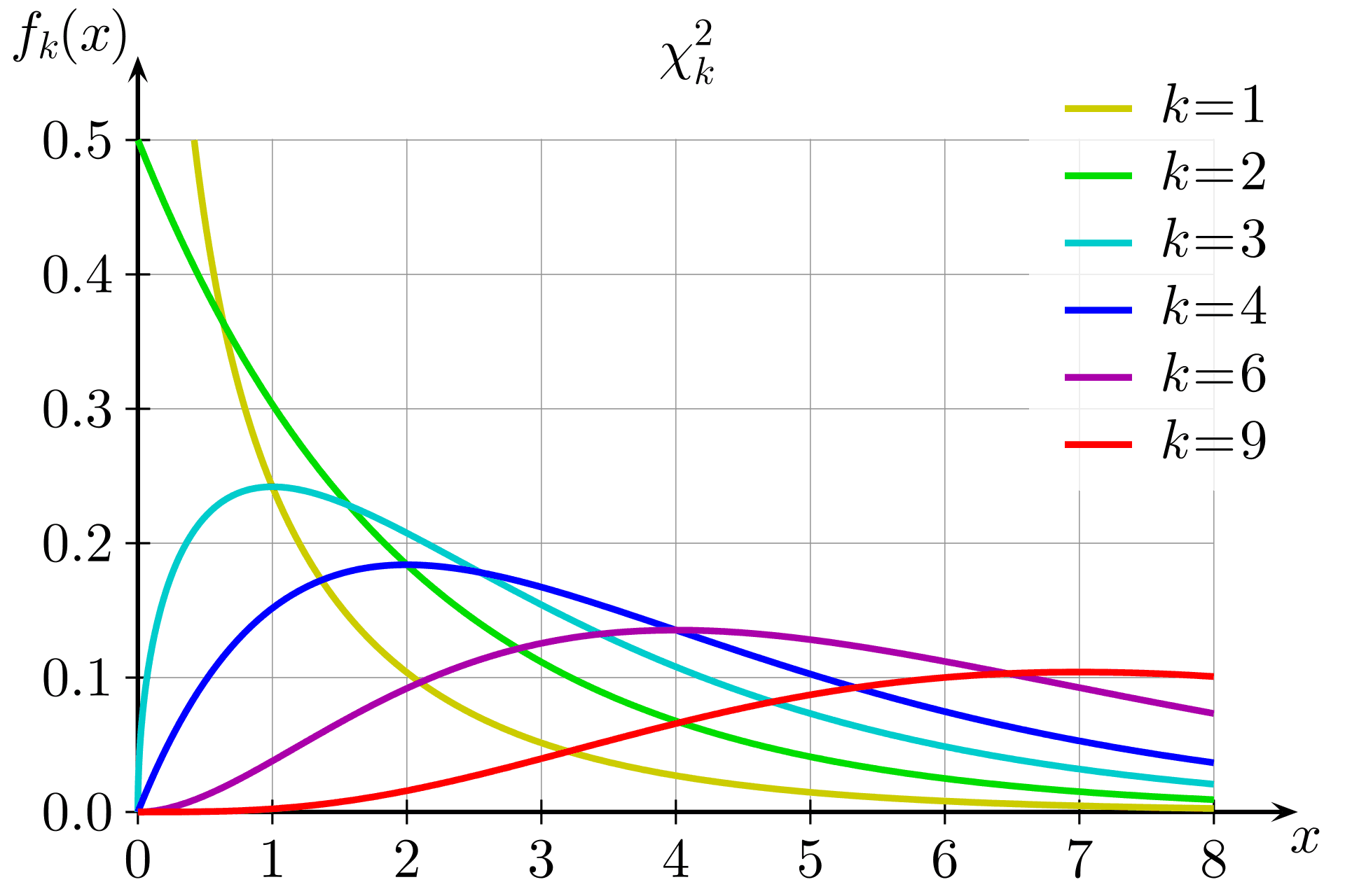
It is intuitive from the look at the p.d.f of Chi-squared distribution $f_{\chi^2_k}(x) = \frac{x^{\frac{k}{2}-1} e^{-x}}{2^k \Gamma(\frac{k}{2})}$ plot that chi-squared probability density function’s maximum is located before its mean $\mathbb{E}\chi^2_k = k$, so by the time it reaches the mean $k$, it is already decreasing. The question is: is it decreasing fast enough - i.e. exponentially?

Gamma function $\Gamma(\frac{k}{2})$ (essentially, $\frac{k}{2}!$ for even $k$) in the denominator of p.d.f. grows faster than $\frac{x^{\frac{k}{2}-1}}{2^k}$ in the numerator starting from some large enough $k$, giving at least an exponential decay on $k$. This follows from Stirling formula: $n! \sim \sqrt{2 \pi n} (\frac{n}{e})^n$ - obviously, $n^n$ outgrows $e^n$. So, at least for large values of relative error $\epsilon$ our statement $p(\chi^2_k \ge k + \epsilon k) \sim e^{-k}$ holds.

Now, we need to prove it for small errors $\epsilon$. What do we do?

Well, the inequality $p(\xi \ge \frac {\mathbb{E}\xi}{\epsilon}) \le ...$ definitely rings a bell. Recall the Markov inequality (a.k.a. Chebyshev’s first inequality in Russian literature):

$p(\xi \ge \epsilon) \le \frac{\mathbb{E}\xi}{\epsilon}$

Unfortunately, its direct application to a chi-square distributed variable doesn’t help, but if we do some tricks with it, we’ll get what we want.

We will potentiate both sides of inequality and introduce a parameter $\lambda$, which we’ll evaluate later. This technique is called Chernoff-Rubin bound:

$p(\chi^2_k \ge (1+\epsilon)k)) = p(\sum \limits_{i=1}^k \xi_i^2 \ge (1+\epsilon)k)) = p(e^{\lambda \cdot \sum \limits_{i=1}^k \xi_i^2} \ge e^{\lambda(1+\epsilon)k})) \le \frac{\mathbb{E}e^{\lambda \cdot \sum \limits_{i=1}^k \xi_i^2}}{e^{\lambda(1+\epsilon)k}}$

$\mathbb{E}e^{\lambda \cdot \xi_i^2} = \frac{1}{\sqrt{2\pi}} \int \limits_{-\infty}^{\infty} e^{\lambda x^2} e^{-\frac{x^2}{2}} dx = \frac{1}{\sqrt{2\pi}} \int \limits_{-\infty}^{\infty} e^{-\frac{x^2 (1-2\lambda)}{2}} dx = \frac{1}{\sqrt{2\pi \frac{1}{1-2\lambda} }} \int \limits_{-\infty}^{\infty} e^{-\frac{x^2}{2 \frac{1}{1-2\lambda}}} dx = \sqrt{\frac{1}{1-2\lambda}}$

$\mathbb{E}e^{\lambda \cdot \sum \limits_{i=1}^k \xi_i^2} = (\mathbb{E}e^{\lambda \cdot \xi_i^2})^k = ({\frac{1}{1-2\lambda}})^{\frac{k}{2}}$

$p(\chi^2_k \ge (1+\epsilon)k)) \le \frac{ ({\frac{1}{1-2\lambda}})^{\frac{k}{2}} }{ e^{\lambda(1+\epsilon)k} } = (1-2\lambda)^{-\frac{k}{2}} e^{-\lambda(1+\epsilon)k}$

The right side is minimized upon $\lambda = \frac{\epsilon}{2(1+\epsilon)}$:

$\frac{\partial{((1-2\lambda)^{-\frac{k}{2}} e^{-\lambda(1+\epsilon)k})}}{\partial{\lambda}} = 2 \cdot \frac{k}{2} \cdot (1-2\lambda)^{-\frac{k}{2}-1} \cdot e^{-\lambda (1+\epsilon)k} - (1+\epsilon)k \cdot (1-2\lambda)^{-\frac{k}{2}} e^{-\lambda (1+\epsilon) k} = 0$

$(1-2\lambda)^{-1} = 1+\epsilon \implies 1-2\lambda = \frac{1}{1+\epsilon} \implies \lambda = \frac{\epsilon}{2(1+\epsilon)}$

Hence, $p(\chi^2_k \ge (1+\epsilon)k) = (1-2\lambda)^{-\frac{k}{2}} e^{-\lambda(1+\epsilon)k} = \frac{1}{1+\epsilon}^{-\frac{k}{2}}e^{-\frac{\epsilon k}{2}} = (1+\epsilon)^{\frac{k}{2}}e^{-\frac{\epsilon k}{2}}$.

Now, use Taylor expansion of $\ln(1+x) = x - \frac{x^2}{2} + \frac{x^3}{3} + \mathcal{o}(x^4) \le x - \frac{x^2}{2} + \frac{x^3}{3}$ and exponentiate it to get: $p(\chi^2_k \ge (1+\epsilon)k) \le e^{\frac{k}{2}(\epsilon - \frac{\epsilon^2}{2} + \frac{\epsilon^3}{3})} e^{-\frac{\epsilon k}{2}} \le e^{-\frac{k}{4}(\epsilon^2 - \epsilon^3)}$.

The proof is analogous for the other bound $p(\chi^2_k \le (1 - \epsilon)k) \le \mathcal{O}(e^{-k})$.

Norm preservation lemma

Recall that $A$ is our d-by-k matrix of random vectors, forming our projection space basis.

Given the results of lemma on chi-squared tails, we shall be able to estimate the probability that the length of a single point is estimated correctly by a random projection, if we manage to prove that ${\Vert \frac{1}{\sqrt{k}} Ax \Vert}^2$ is a Chi-square-distributed random variable. Then this result will follow:

$p((1-\epsilon) {\Vert x \Vert}^2 \le {\Vert \frac{1}{\sqrt{k}} Ax \Vert}^2 \le (1+\epsilon) {\Vert x \Vert}^2) \ge 1 - 2e^{-\frac{k}{4}(\epsilon^2-\epsilon^3)}$

So, how to show that ${\Vert \frac{1}{\sqrt{k}} Ax \Vert}^2 \sim \chi^2_k$?

First, note that in the projection vector $y = {Ax}$ each coordinate $y_i$ is a weighted sum of gaussian random variables and is itself a gaussian random variable.

Its expectation is, obviously, 0. Its variance, however, is unknown. Let us show that it is 1:

$\mathbb{E}y_i^2 = \mathbb{E}((\xi_{i,1}x_1 + \xi_{i,2}x_2 + ... + \xi_{i, d}x_d))^2 = \underbrace{\mathbb{E}(x_1^2 \xi_1^2 + x_2^2 \xi_2^2 + ... + x_d^2 \xi_d^2)}_{{\Vert x \Vert}^2} + \mathbb{E}(\sum_{i,j} x_i x_j \xi_i \xi_j) = {\Vert x \Vert}^2 + \sum_{i,j} x_i x_j \cancel{\mathbb{E}\xi_i} \cancel{\mathbb{E}\xi_j} = {\Vert x \Vert}^2$,

where $\xi_{i,j} \sim \mathcal{N}(0, 1)$ are individual standard normal random variables that are the elements of matrix A.

Now, if we sum over coordinates $y_i$ of the projection vector, we get the desired result:

$\Vert \frac{1}{\sqrt{k}}y \Vert^2 = \frac{1}{k}\sum \limits_i^k y_i^2 = {\Vert x \Vert}^2$.

Johnson-Lindenstrauss theorem

Johnson-Lindenstrauss theorem follows from the norm preservation lemma immediately.

If you have $n$ points, you have $n^2$ distances between them (including distance from a point to itself). The chance that none of the distances is wrong, thus, is

$p(\text{any of } n^2 \text{distances is very wrong}) \le 1 - (1 - p((1-\epsilon) {\Vert x \Vert}^2 \le {\Vert \frac{1}{\sqrt{k}} Ax \Vert}^2 \le (1+\epsilon) {\Vert x \Vert}^2)^{n^2} \approx 1 - 1 + 2 n^2 e^{-\frac{k}{4}(\epsilon^2-\epsilon^3)} = 2 n^2 e^{-\frac{k}{4}(\epsilon^2-\epsilon^3)}$.

Thus, you need $k \ge \frac{C \cdot \log n}{\epsilon^2}$ to keep this probability as small as you prefer, where $C$ is some constant.

Bonus: inner product (angles) preservation

Norm preservation lemma above guarantees not only preservation of distances, but of angles as well.

Assume that $u$ and $v$ are two vectors, and $\frac{1}{\sqrt{k}}Au$ and $\frac{1}{\sqrt{k}}Av$ are their random projections. Then:

$(1-\epsilon) {\Vert u - v \Vert}^2 \le {\Vert \frac{1}{\sqrt{k}}A(u-v) \Vert}^2 \le (1+\epsilon) {\Vert u - v \Vert}^2$

$(1-\epsilon) {\Vert u + v \Vert}^2 \le {\Vert \frac{1}{\sqrt{k}}A(u+v) \Vert}^2 \le (1+\epsilon) {\Vert u + v \Vert}^2$

Subtract one inequality from the other (note that this leads to inversion of sides of double inequalities in the subtracted inequality):

${\Vert \frac{1}{\sqrt{k}}A(u+v) \Vert}^2 - {\Vert \frac{1}{\sqrt{k}}A(u-v) \Vert}^2 = 4 \frac{1}{k} (Au, Av) \ge (1-\epsilon) {\Vert u + v \Vert}^2 - (1+\epsilon) {\Vert u - v \Vert}^2 = 4(u,v) - 2 \epsilon (\Vert u \Vert^2 + \Vert v \Vert^2) \ge 4(u,v) - 4 \epsilon$

So, as a result we get: $(u,v) - \epsilon \le \frac{1}{k} (Au, Av) \le (u,v) + \epsilon$ with probability $1 - 2e^{-\frac{k}{4}(\epsilon^2-\epsilon^3)}$ or higher.

Not only Gaussian

Here we used gaussian random variables as elements of our random projection matrix $A$, followed by analysis of Chi-squared distribution.

But note that when the number of degrees $k$ approaches 100, Chi-square converges to Gaussian very closely, and relative error near mean is decaying as an exponential function of $k$ as $k$ increases. Seems like the convergence rate of central limit theorem could be a valuable tool here for other distribution types.

So in that regard it doesn’t make much difference, which random variables we take as elements of $A$, Gaussian or not. Another purpose Gaussians served here, was their useful property that a weighted sum of Gaussian random variables is Gaussian itself, which might not be the case for other distributions. But as soon as this property holds, we can use other distribution types for random projections.

There is a natural way to define a subset of distributions that would fit: a distribution $\xi$ is called sub-Gaussian with a parameter $\lambda$, if $\mathbb{E}e^{\lambda \xi} \le e^{\lambda x^2}$ for all real $x$. As you recall, we used this $e^{\lambda x^2}$ in our Chernoff bound. A popular alternative is to use Bernoulli random variables with random signs {-1, 1} instead.

Tightness of estimate

Throughout 2014-2021 in a series of papers Larson and Nelson and Alon and Klartag (see references) showed that the bound $\mathcal{O}(\frac{\log n}{\epsilon^2})$, given by Lindenstrauss-Johnson is optimal for any linear or even non-linear projection.

The papers are fairly technical, they employ approaches from classical functional analysis (like coverages with balls and Minkowski functional) and coding theory (such as Reed-Solomon codes). See references section.

Applications

Manifold learning/multidimensional scaling

Johnson-Lindenstrauss suggests a way to look at your t-SNE/UMAP plots. As 2D or 3D is definitely not enough for an accurate depiction of the multidimensional distances, don’t trust them in your plots.

Statements like “point B is 2 times farther from point A than point C” make no sense - the distances could’ve been distorted and with different parameters of the projection you might get a picture, where point C is 2 times farther form point A that point B.

The only thing you can more or less trust in t-SNE is the notion of neighbourhood: if points A and B are very close on t-SNE plot, they are very close in the original multidimensional space. As an example, see a recent crusade of the adorable Lior Pachter against t-SNE and UMAP.

Rule of thumb for an autoencoder latent space

If you’re not sure about the dimensionality of the latent space of your autoencoder, such as VAE, Johnson-Lindenstrauss suggests that $k = \sim 100$ is a good rule of thumb. It is small enough and preserves distances well enough.

Compressed sensing

Johnson-Lindenstrauss provides an excellent intuition on how to achieve a sparse space in compressed sensing. I’ll dedicate a whole separate post to this beautiful mathematical theory.

References

• https://home.ttic.edu/~gregory/courses/LargeScaleLearning/lectures/jl.pdf - proof outline number 1
• https://cseweb.ucsd.edu/~dasgupta/papers/jl.pdf - proof outline number 2
• https://en.wikipedia.org/wiki/Johnson%E2%80%93Lindenstrauss_lemma
• http://www.cs.cmu.edu/afs/cs/academic/class/15750-s19/OldScribeNotes/lecture23.pdf - a good overview of the state of the field, generalizations and recent results
• https://arxiv.org/pdf/1610.00239.pdf - Alon and Klartag paper on JL optimality
• https://arxiv.org/pdf/1411.2404.pdf, https://cs.au.dk/~larsen/papers/jl_transform.pdf - Larsen and Nelson paper on proof of optimality of JL for linear maps
• https://arxiv.org/pdf/1609.02094.pdf - Larsen and Nelson paper with proof of optimality of JL estimate for any map
• https://arxiv.org/pdf/2107.06626.pdf - most recent Larsen paper on JL optimality

Written by Boris Burkov who lives in Moscow, Russia, loves to take part in development of cutting-edge technologies, reflects on how the world works and admires the giants of the past. You can follow me in Telegram