Quadratic programming

Problem statement

General case of quadratic programming problem is stated as follows.

Suppose, that you have a vector of multiple variables $\bf{x} = \begin{pmatrix} x_1 \\ x_2 \\ ... \\ x_n \end{pmatrix}$. given by a quadratic form + a linear bias

You have a function of those variables, which is a sum of quadratic term and linear term $f(x) = \frac{1}{2} {\bf x}^T Q {\bf x} - {\bf x}^T \bf{b}$.

Here quadratic term is given by a quadratic form $Q = \begin{pmatrix} q_{1,1} && q_{1,2} && ... && q_{1,n} \\ q_{2,1} && q_{2,2} && ... && q_{2,n} \\ ... && ... && \ddots && ... \\ q_{n,1} && q_{n,2} && ... && q_{n,n} \end{pmatrix}$.

The linear term is given by a dot product of $\bf{x}$ with bias weights vector: $\bf{b} = \begin{pmatrix} b_1 \\ b_2 \\ ... \\ b_n \end{pmatrix}$.

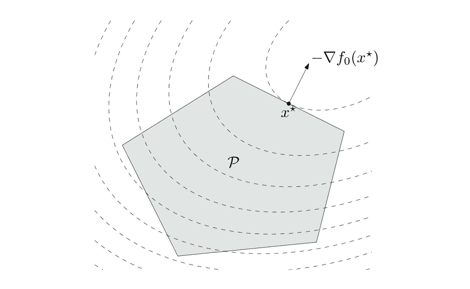
We also have a set of $m$ constraints in the form of linear inequalities, that delimit the possible solution to a convex subset of your input subspace:

$A \bf{x} \le \bf{c}$, where $A = \begin{pmatrix} a_{1,1} && a_{1,2} && ... && a_{1,n} \\ ... \\ a_{m,1} && a_{m,2} && ... && a_{m,n} \end{pmatrix}$ and $\bf{c} = \begin{pmatrix} c_1 \\ c_2 \\ ... \\ c_m \end{pmatrix}$

These constraints are called Karush-Kuhn-Tucker.

Solution in case of strict equality

In case Karush-Kuhn-Tucker conditions are strict equalities, not inequalities, the solution becomes fairly straightforward.

We shall just apply Lagrange multiplier method and find the conditional minimum of our system on variables $x_i$ and $\lambda_i$, where $\Lambda = \begin{pmatrix} \lambda_1 \\ \lambda_2 \\ ... \\ \lambda_m \end{pmatrix}$ are Lagrange multipliers.

Just add equations $\lambda_i A_i \bf{x}= \lambda_i c_i$ to $f(\bf{x}) = \frac{1}{2} \bf{x}^T Q \bf{x} + \bf{x}^T \bf{b}$ and take the partial derivatives on $x_i$, equating them to zero:

$\frac{\partial (\frac{1}{2}(x_i q_{i,1} x_1 + x_i q_{i,2} x_2 + ... + x_i q_{i,n} x_n) - (b_1 x_1 + ... b_n x_n) + \lambda_1 (a_{1,1} x_1 + ... + a_{1,n} x_n) + ... + \lambda_m (a_{m,1} x_1 + ... + a_{m,n} x_n))}{\partial x_i} = 0 \implies$

$\implies q_{i,1} x_1 + ... + q_{i,n} x_n - b_i + \lambda_1 a_{1,i} + \lambda_2 a_{2,i} + ... + \lambda_m a_{m,i} = 0$

and also we have the equations $a_{i,1} x_1 + a_{i,2} x_2 + ... + a_{i,n} x_n = c_i$ themselves.

Thus, solution takes form of a system of $n+m$ linear equations with $n+m$ variables ($\bf{x}$ and $\bf{\lambda}$):

$\begin{pmatrix} q_{1,1} && ... && q_{1,n} && a_{1,1} && ... && && a_{m,1} \\ ... \\ q_{n,1} && ... && q_{n,n} && a_{1,n} && ... && && a_{m,n} \\ a_{1,1} && ... && a_{1,n} && 0 && ... && 0 \\ ... \\ a_{m,1} && ... && a_{m,n} && 0 && ... && 0 \end{pmatrix} \begin{pmatrix} x_1 \\ ... \\ x_n \\ \lambda_1 \\ .... \\ \lambda_m \end{pmatrix} = \begin{pmatrix} b_1 \\ ... \\ b_n \\ c_1 \\ ... \\ c_m \end{pmatrix}$

or, in short notation:

$\begin{pmatrix} Q && A^T \\ A && 0 \end{pmatrix} \begin{pmatrix} \bf{x} \\ \bf{\lambda} \end{pmatrix} = \begin{pmatrix} \bf{b} \\ \bf{c} \end{pmatrix}$

Thus, solution is straightforward.

References

• https://www.math.uh.edu/~rohop/fall_06/Chapter3.pdf - great paper on square programming techniques
• http://www.apmath.spbu.ru/cnsa/pdf/monograf/Numerical_Optimization2006.pdf - a magnum opus on numerical optimization by Wright and Nocedal
• http://www.ccgalberta.com/ccgresources/report13/2011-113_comparing_optimization_methods.pdf - on sequential quadratic programming compared to gradient descent and interior point method
• http://www.mathnet.ru/links/b3b151bdcecb5b2554cc126c89a4373e/zvmmf5189.pdf - soviet paper on solution of quadratic programming
• https://ru.wikipedia.org/wiki/%D0%9A%D0%B2%D0%B0%D0%B4%D1%80%D0%B0%D1%82%D0%B8%D1%87%D0%BD%D0%BE%D0%B5_%D0%BF%D1%80%D0%BE%D0%B3%D1%80%D0%B0%D0%BC%D0%BC%D0%B8%D1%80%D0%BE%D0%B2%D0%B0%D0%BD%D0%B8%D0%B5 - Russian wikipedia
• https://en.wikipedia.org/wiki/Taylor%27s_theorem - Taylor’s series derivation in univariate and multivariate cases

Written by Boris Burkov who lives in Moscow, Russia, loves to take part in development of cutting-edge technologies, reflects on how the world works and admires the giants of the past. You can follow me in Telegram