Written by Boris Burkov who lives in Moscow, Russia, loves to take part in development of cutting-edge technologies, reflects on how the world works and admires the giants of the past.
Intro to the Extreme Value Theory and Extreme Value Distribution
April 30, 2023 167 min read
Quite often in mathematical statistics I run into Extreme Value Distribution - an analogue of Central Limit Theorem, which describes the distribution of maximum/minimum, observed in a series of i.i.d random variable tosses. This is an introductory text with the basic concepts and proofs of results from extreme value theory, such as Generalized Extreme Value and Pareto distributions, Fisher-Tippett-Gnedenko theorem, von Mises conditions, Pickands-Balkema-de Haan theorem and their applications.
Contents:
Problem statement and Generalized Extreme Value distribution
Type I: Gumbel distribution
Type II: Frechet distribution
Type III: Inverse Weibull distribution
Fisher-Tippett-Gnedenko theorem
Examples of convergence
General approach: max-stable distributions as invariants/fixed points/attractors and EVD types as equivalence classes
Khinchin’s theorem (Law of Convergence of Types)
Necessary conditions of maximium stability
Fisher-Tippett-Gnedenko theorem (Extreme Value Theorem)
Distributions not in domains of attraction of any maximum-stable distributions
Von Mises sufficient conditions for a distribution to belong to a type I, II or III
Pre-requisites from survival analysis
Von Mises conditions proof
Generalizations of von Mises condition for Type I EVD: auxiliary function and von Mises function
Necessary and sufficient conditions for a distribution to belong to a type I, II or III
Pre-requisites from Karamata’s theory of slow/regular/Г-/П- variation
Necessary and sufficient conditions of convergence to Types II or III EVD
Necessary and sufficient conditions of convergence to Type I EVD
Residual life time
Generalized Pareto distribution
Residual life time problem
Pickands-Balkema-de Haan theorem (a.k.a. Second Extreme Value Theorem)
Order statistics and parameter estimation
Order statistics
Hill’s estimator
Pickands’ estimator
Other estimators
Summary and examples of practical application
Examples of Type I Gumbel distribution
Examples of Type II Frechet distribution
Examples of Type III Inverse Weibull distribution
Concluding remarks
1. Problem statement and Generalized Extreme Value distribution
One of the most famous results in probabilities is Central Limit Theorem, which claims that sum of n→∞ i.i.d. random variables ξi
after centering and normalizing converges to Gaussian distribution.
Now, what if we ask a similar question about maximum of those n→∞ i.i.d. random variables instead of sum? Does it converge to any distribution?
Turns out that it depends on the properties of the distribution ξi, but not much really. Regardless of the distribution
of ξi the distribution of maximum of n random variables ξi is:
Gγ(x)=exp(−(1+γx)−γ1)
This distribution is called Generalized Extreme Value Distribution. Depending on the coefficient γ it can take
one of three specific forms:
Type I: Gumbel distribution
If γ→0, we can assume that k=γ1→∞. Then generalized EVD converges to a
doubly-exponential distribution (sometimes this is called a law of double logarithm) by definition of e=(1+k1)k and ex=(1+k1x)k:
This is Gumbel distribution, it oftentimes occurs in various areas, e.g. bioinformatics, describing the distribution
of longest series of successes in coin tosses in n experiments of tossing a coin 100 times.
It is often parametrized by scale and center parameters. I will keep it centered here, but will add shape parameter λ:
F(x)=e−e−λx, or, in a more intuitive notation F(x)=ex/λe1.
It is straightforward to derive probability density function f(x) from here:
f(x)=∂x∂F=−e−λx⋅(−λ1)⋅e−e−λx=λ1e−λx+e−λx.
import math
import numpy as np
import matplotlib.pyplot as plt
scale =1# Generate x values from 0.1 to 20 with a step size of 0.1
x = np.arange(-20,20,0.1)# Calculate y values
gumbel_cdf = math.e**(-math.e**(-(x/scale)))
gumbel_pdf =(1/ scale)* np.exp(-( x/scale + math.e**(-(x / scale))))# Create the figure and axis objects
fig, ax = plt.subplots(figsize=(12,8), dpi=100)# Plot cdf
ax.plot(x, gumbel_cdf, label='cdf')# Plot pdf
ax.plot(x, gumbel_pdf, label='pdf')# Set up the legend
ax.legend()# Set up the labels and title
ax.set_xlabel('x')
ax.set_ylabel('y')
ax.set_title('Plot of Gumbel pdf and cdf')# Display the plot
plt.show()
Gumbel distribution plot, scale = 1.
Type II: Frechet distribution
If γ>0, let us denote k=γ1 (k > 0), y=λ⋅(1+γx), where k is called
shape parameter and λ - scale parameter. Then distribution takes the shape:
Gγ(x)=exp(−(1+γx)−γ1)=exp(−(λy)−k).
To make it more intuitive, I’ll re-write cdf in the following way: F(x)=e(xλ)k1.
This is Frechet distribution. It arises when the tails of the original cumulative distribution function
Fξ(x) are heavy, e.g. when it is Pareto distribution.
Let us derive the probability density function for it:
import math
import numpy as np
import matplotlib.pyplot as plt
shape =2# alpha
scale =2# beta# Generate x values from 0.1 to 20 with a step size of 0.1
x = np.arange(0,20,0.1)# Calculate y values
frechet_cdf = math.e**(-(scale / x)** shape)
frechet_pdf =(shape / scale)*((scale / x)**(shape +1))* np.exp(-((scale / x)** shape))# Create the figure and axis objects
fig, ax = plt.subplots(figsize=(12,8), dpi=100)# Plot cdf
ax.plot(x, frechet_cdf, label='cdf')# Plot pdf
ax.plot(x, frechet_pdf, label='pdf')# Set up the legend
ax.legend()# Set up the labels and title
ax.set_xlabel('x')
ax.set_ylabel('y')
ax.set_title('Plot of Frechet distribution pdf and cdf')# Display the plot
plt.show()
Frechet distribution plot, scale = 1, shape = 1.
Type III: Inverse Weibull distribution
If γ<0, let us denote k=−γ1 (k > 0, different kinds of behaviour are observed at 0<k<1, k=1 and k>1), y=λ(1+γx).
Then distribution takes the shape:
Gγ(x)=exp(−(1+γx)−γ1)=exp(−(λy)k).
Gγ(x)={exp(−(λx)k),x≤01,x>0.
This is Inverse Weibull distribution. Its direct counterpart (Weibull distribution) often occurs in
survival analysis as a hazard rate function. It also arises in mining - there it
describes the mass distribution of particles of size x and is closely connected to Pareto distribution. We shall
discuss this connection later.
Generalized extreme value distribution converges to Inverse Weibull, when distribution of our random variable ξ is bounded.
E.g. consider uniform distribution ξ∼U(0,1). It is clear that the maximum of n uniformly distributed
variables will be approaching 1 as n→∞. Turns out that the convergence rate is described by Inverse Weibull
distribution.
To make it more intuitive, we can re-write the cdf as F(x)={e(λ−x)k1,x≤01,x>0.
Derive from cumulative distribution function F(x)=exp(−(λ−x)k) the probability density function:
import math
import numpy as np
import matplotlib.pyplot as plt
shape =2# alpha
scale =2# beta# Generate x values from 0.1 to 20 with a step size of 0.1
x = np.arange(-20,0,0.1)# Calculate y values
inverse_weibull_cdf = math.e**(-(-x/scale)** shape)
inverse_weibull_pdf =(shape / scale)*((-x / scale)**(shape -1))* np.exp(-((-x / scale)** shape))# Create the figure and axis objects
fig, ax = plt.subplots(figsize=(12,8), dpi=100)# Plot cdf
ax.plot(x, inverse_weibull_cdf, label='cdf')# Plot pdf
ax.plot(x, inverse_weibull_pdf, label='pdf')# Set up the legend
ax.legend()# Set up the labels and title
ax.set_xlabel('x')
ax.set_ylabel('y')
ax.set_title('Plot of Inverse Weibull pdf and cdf')# Display the plot
plt.show()
Extreme Value Theorem is a series of theorems, proven in the first half of 20-th century. They claim that
maximum of several tosses of i.i.d. random variables converges to just one of 3 possible distributions,
Gumbel, Frechet or Weibull.
Here I will lay out the outline of the proof with my comments. The proof includes introduction of several
technical tools, but I will comment on their function and rationale behind each of them.
Consider a random variable Mn, which describes the distribution of maximum of ξi, i∈1..n
p(Mn≤x)=i=1∏np(ξi≤x)=Fn(ξi≤x).
Similarly to the Central Limit Theorem, a convergence theorem might be applicable to the distribution of a
normalized random variable Mn rather than the non-normalized:
p(anMn−bn≤x)=p(Mn≤anx+bn)=Fn(anx+bn)
We aim to show that for some series of constants ai and bi
Fn(anx+bn) as n→∞ converges in distribution to some distribution G(x): Fn(anx+bn)wn→∞G(x).
Now I will provide several examples and then informally describe the proof outline, before introducing the mathematical formalism.
Examples of convergence
Let us start with simple examples of convergence to types I and II to get a taste of how convergence to maxima works.
Example 2.1. Convergence of maximum of i.i.d. exponential random variables to Gumbel distribution
I’ll never believe that a horse and a wagon age in the same way.
- Alex Comfort (as quoted by Vladimir P. Skulachev)
Consider a wagon with an exponentially-distributed life time. For instance, assume that the probability for a wagon to break down every
year is 1/e.
Then let ξ random variable be its lifetime and its cdf be:
Fξ(x)=p(ξ≤x)=1−e−x
Given n→∞ wagons, what’s the distribution of lifetime of the longest living one?
We see that this is almost standard Gumbel distribution (type I EVD).
In order to get the stadard one, we need to consider a shifted random variable p(maxξi≤anx+bn) by choosing an=1, bn=logn, so that we
get:
Fn(x+logn)=(1−e−(x+logn))n=(1−ne−x)n→exp(−e−x).
Example 2.2. Convergence of maximum of i.i.d. Pareto random variables to Frechet distribution
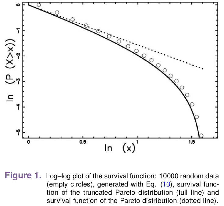
Consider another example: Pareto distribution. It describes the distribution of wealth (e.g. fraction of people, having net worth above x),
sizes of cities (e.g. fraction of cities with a population greater than x), sizes of orders on an exchange (e.g. fraction of orders of size
greater than x), number of Telegram channels with more than x subsribers. Here is its cdf:
Fξ(x)=p(ξ≤x)=1−(xx0)α
It is often convenient to depict it in log-log coordinates because ln(1−Fξ(x))=γ(lnx0−lnx):
Pareto distribtuion also describes the distribution of life time of memes, comedy shows etc. This phenomenon is
known as Lindy effect. With a little calculation one can show that expected lifetime of a comedy
show equals to the time it’s already been around, which leads to Pareto distribution of its cdf.
Again, let us consider the distribution of maximum lifetime of the comedy shows then:
We see that it converges to Frechet (EVD type II) distribution.
Example 2.3. Convergence of minimum/maximum of i.i.d. Weibull/inverse Weibull random variables to Weibull/inverse Weibull distribution
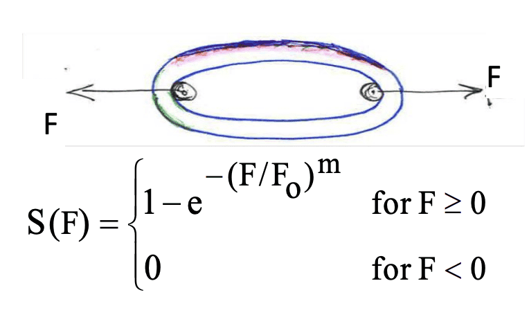
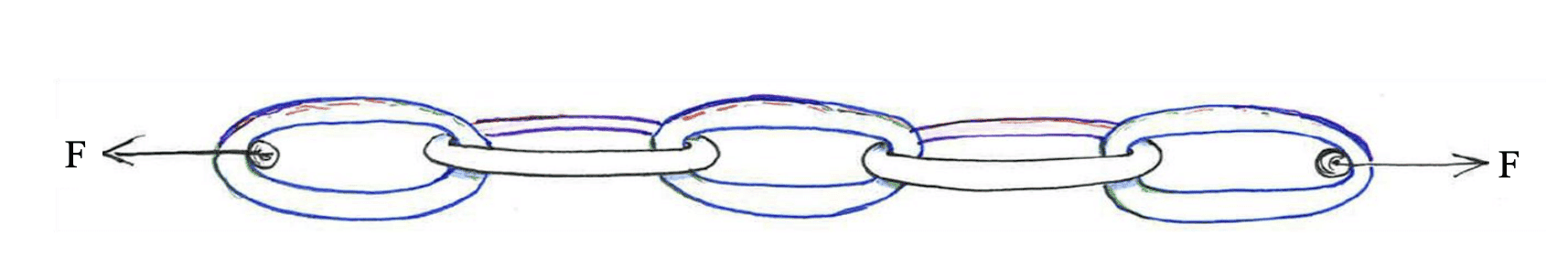
Consider a single link of a chain, the strength of which is described by a Weibull distribution Fξ(x)=p(ξ≤x)=1−e−(x0x)m:
In this specific application of Weibull distribution we may say that the strength of a link S(F) is the probability that it does not break under application of force F (sorry for the duplication of symbol F in the notation, used as both cdf and force).
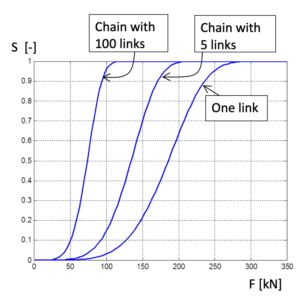
Then we can show that strength of the whole chain is also described by Weibull distribution, as the chain is as strong as its weakest link:
We see that the whole chain’s strength also follows the Weibull distribution, but with somewhat altered parameter:
Similarly, we may consider a zipper, where strength of a zipper is the strength of the hardest-to-open element. Hence, strength of a zipper and
of each element of it is described by inverse Weibull distribution:
Later on we will introduce the concept of max-stable/min-stable distributions, i.e. such distributions that maximum/minimum of them follows the
same distribution. With this example we can already see that Weibull distribtuion is min-stable and inverse Weibull distribution is max-stable.
In these examples we used the same argument: (1−n1−F(x))nne−(1−F(x)).
It might seem that we can substitute any distribution as (1 - F(x)) and make the distribution of maximum e−(1−F(x)) to take almost any shape.
However, it turns out that this intuition is wrong, as there are just 3 possible shapes of Extreme Value Distribution.
Let’s see, how (counter-intuitively) the maximum of i.i.d. Gaussian random variables converges to Gumbel.
Example 2.4. Convergence of maximum of i.i.d. Gaussian random variables to Gumbel distribution
Step 1. Integration in parts
Let us consider the cdf of normal distribution F(x)=p(ξ≤x)=2π1−∞∫xe−t2/2dt=1−p(ξ≥x)=1−2π1x∫∞e−t2/2dt.
Do integration in parts: 2π1x∫∞e−t2/2dt=2π1xe−2x2−2π1x∫∞t2e−t2/2dt
Recall that we are interested in maximum of anx+bn, not just x.
Hence, we want to study the behaviour of 2π1anx+bne−2(anx+bn)2 and to show that 2π1anx+bne−2(anx+bn)2∼ne−x.
Step 2. Split result in two multipliers, select an
Let us use our freedom to choose an and bn.
First let us choose an, while letting bn→∞ (we will choose a specific bn at a later stage).
By evaluating the square of anx+bn we’ve managed to come up with 2 multipliers. First of them contains e−x, which is required for convergence to Gumbel distribution. Note that as bn→∞, first term converges to e−x:
x/bn2+1e−x2/2bn2e−xbn→∞e−x
The second term bne−bn2/2 will produce 1/n that we need to obtain (1−F(x)/n)n.
Step 3. Select bn
Choose bn=F−1(1−1/n), so that:
bne−bn2/2→1−F(F−1(1−1/n))=n1
Hence, we end up having F(anx+bn)→1−e−x/n, where bn=F−1(1−1/n) and an=bn1.
Then p(maxξi≤anx+bn)=p(ξi≤anx+bn)n=(1−e−x/n)n=e−e−x.
This is just one example of a distribution, for which it doesn’t appear at the first glance that its maximum would
converge to one of 3 types of EVD, but its maximum actually does converge to Type I. We shall prove as a theorem that for
i.i.d. random variables from any distribution there are just 3 options for their maximum to converge to. Let’s first
discuss the general approach of how this could be shown, and then will proceed with a formal proof.
General approach: max-stable distributions as invariants/fixed points/attractors and EVD types as equivalence classes
I assume that all three types of Extreme Value Distribution were first discovered experimentally. Later statisticians
came up with a proof that EVD can converge to just one of three possible types of distributions and no other types of
EVD can exist. Finally, they came up with criteria for a distribution to belong to each type.
Design of this proof is similar to many other proofs. I will outline it informally here:
Assume that as the number of random variables n→∞ increases, approaching infinity, the distribution of the
observed maximum approaches some type of distribution. Then such a distribution type can be considered as an invariant
or attractor or fixed point, similar to many other mathematical problems. For instance, eigenvectors are fixed points
of matrix multiplication. E.g. matrix eigenvector, multiplied by a matrix, results in itself, multiplied by a scalar. Or
no matter how many times you take a derivative of ekx, you get ekx, multiplied by a scalar k.
Similarly, maximum-stable distributions are invariant objects. Those are distributions, maximum of i.i.d. variables
of which converges to themselves, no matter how many more i.i.d. random variables you toss. E.g. if for one
Gumbel-distributed random variable ξ we know that pξ(a1M1−b1≤x)=e−e−x, for n→∞
Gumbel-distributed random variables the maximum of ξ1..ξn still is Gumbel-distributed (after centering and
normalizing them by some numbers an, bn): pMn(anMn−bn≤x)=e−e−x.
Ok. Then after we established that there are some distributions, for which maximum of n→∞ centered and normalized
i.i.d. variables produces a random variable with the same distribution, how do we show that all distributions converge
to one of them?
We’ll use another classical mathematical tool: equivalence classes and equivalence relation. For instance,
odd numbers and even numbers form two equivalence classes under operation of modulo 2. Odd numbers are equivalent to
each other in terms of producing remainder 1 (e.g. 3∼5, where ∼ is equivalence relation of modulo 2), and even
numbers are equivalent in terms of producing remainder 0.
Similarly, we will show that types of EVD form equivalence classes under the operation of finding maximum of n→∞
i.i.d. random variables with any distribution, and as a result all the distributions converge to one of those types. E.g.
Pareto’s distribution is equivalent to Cauchy distribution under equivalence relation of convergence of maximum of
n→∞ Pareto/Cauchy i.i.d’s to the same maximum stable type II (Frechet) EVD.
Now that I’ve laid out the plan of the proof, it is time to get into technicalities. I will formally introduce the concepts
I mentioned above and prove some lemmas about their relatedness.
Definition 2.1: Max-stable cumulative distribution function
G is max-stable if for all n∈1..N and for all x there exists {an},{bn}⊂R+ such that for all
x∈RG(x)=Gn(anx+bn).
Definition 2.2: Domain of attraction
If F is a cdf, then F is in the domain of attraction (for maxima) of G, and it is written F∈D(G),
when there exist sequences {an},{bn}⊂R+ such that Fn(anx+bn)wn→∞G(x).
Definition 2.3: Type of convergence
If G∗(x) is another non-degenerate cdf, we say that G and G∗ have the same type if for all x there exist
a>0 and b∈R such that for every x ∈ R G∗(ax+b)=G(x).
Khinchin’s theorem (Law of Convergence of Types)
Aleksandr Yakovlevich Khinchin
Lemma 2.1: Khinchin’s theorem (law of Convergence of Types)
Suppose that we have a sequence of distribution functions {Fn} (e.g. the distributions of maximum of random variable ξi in n experiments).
Let those distribution functions upon n→∞ converge to a certain distribution G(x): Fn(anx+bn)wn→∞G(x). Then we have two series of constants {an},{bn}.
Suppose there is another distribution function H(x) such that the sequence of distributions Fn(αnx+βn) converges to that function: Fn(αnx+βn)wn→∞H(x) and there is a different pair of series {αn},{βn}.
Then H(x)=G(Ax+B) and A=anαn, B=anβn−bn.
Proof:
Consider two distribution functions G(x) and H(x), such that for every x: y=F(ax+b) and y=F(αx+β).
Denote y=F(ax+b)→G(x). Then F−1(y)=ax+b and x=aF−1(y)−b→G−1(y).
Similarly y=F(αx+β)→H(x) and F−1(y)=αx+β and x=αF−1(y)−β→H−1(y).
Now choose two points: x1, corresponding to y1, and x2, corresponding to y2 and subtract x1 and x2 from each other:
x1−x2=aF−1(y1)−F−1(y2)→G−1(y1)−G−1(y2)
Apply the same for H−1:
x1−x2=αF−1(y1)−F−1(y2)→H−1(y1)−H−1(y2)
Which results in H−1(y1)−H−1(y2)G−1(y1)−G−1(y2)→aα=A.
Substitute α=A⋅a into H−1(y)→x=A⋅aF−1(y)−β and A⋅H−1(y)→A⋅x=aF−1(y)−β.
On the other hand we recall that G−1(y)→x=aF−1(y)−b. Subtracting these, we get: A⋅H−1(y)−G−1(y)→aF−1(y)−β−aF−1(y)−b=ab−β or aβ−b=B→G−1(y)−A⋅H−1(y).
Hence, G−1(y)→A⋅H−1(y)+B.
Lemma 2.2: Necessary condition of maximum-stability
Given G a non-degenerate cdf:
G is max-stable if and only if there exists a sequence {Fn} of cdf ’s and sequences
{an}⊂R+, {bn} such that for all k∈NFn(ankx+bnk)wn→∞G1/k(x)
D(G)=0 if and only if G is max-stable. In that case, G∈D(G).
Proof:
Proposition 1 direct statement: if G is max-stable, there exists {Fn} such that …
If G is max-stable, then by definition for every n∈N there exist an, bn, such that Gn(anx+bn)=G(x).
Define Fn=Gn. Then Fnk(ankx+bnk)=Gnk(ankx+bnk)=G. We arrive at the direct statement.
Proposition 1 reverse statement: if G is max-stable, there exists {Fn} such that …
Let us proof the reverse statement: suppose that the sequences {Fn}, {an}, {bn} exist, such that for all k∈N:
Fn(ankx+bnk)wn→∞G1/k(x)
Then consider k=1 and k=2:
Fn(anx+bn)wn→∞G(x) and Fn(a2nx+b2n)wn→∞G1/2(x)
By Khinchin’s lemma there exists G(α2x+β2)=G1/2(x).
Similarly, for every other k: G(αkx+βk)=G1/k(x) or Gk(αkx+βk)=G(x), which is the
definition of max-stability.
Proposition 2 direct statement:
The proof is self-evident: if G is max-stable, Gn(anx+bn)=G(x), and G∈D(G) by defintion.
Proposition 2 reverse statement:
Assume F∈D(G), i.e. Fn(anx+bn)wn→∞G(x).
For all k∈N we have Fnk(ankx+bnk)wn→∞G(x).
Hence, Fn(ankx+bnk)wn→∞G1/k(x)
This makes G and Gk fit for the conditions of previous result, proving that G is max-stable.
Corollary 2.1:
Let G be a max-stable cdf. Then there exist functions a(s)>0 and b(s) such that for all x∈R, for all s>0,
Gs(a(s)x+b(s))=G(x).
Corollary is self-evident from inversion of indices s=k1.
Fisher-Tippett-Gnedenko theorem (Extreme Value Theorem)
Sir Ronald Aylmer Fisher
Leonard Henry Caleb Tippett
Boris Vladimirovich Gnedenko
Theorem 2.1: Fisher-Tippett-Gnedenko theorem (Extreme Value Theorem)
Let ξi be a sequence of i.i.d. random variables.
If there exist constants an>0, bn∈R and some
non-degenerate cumulative distribution function G such that anMn−bn∼G, then G is one of these:
Here we give the proof of Fisher-Tippett-Gnedenko theorem without introducing any additional pre-requisites and
intermediate constructs. Because of that it might look like black magic now. It is not clear, how anyone could’ve come
up with this proof.
However, later on in parts 3 and 4 we will give the definitions of tail quantile function and tools from Karamata’s
theory of slow/regular variation.
If you revisit this proof afterwards, you will notice that we’re making use of those tools, without naming them explicitly.
Step 1.
Consider double negative logarithm of max-stable distribution G(a(s)x+b(s))s=G(x).
We can swap y and z in previous equation, settings y=z and z=y:
ψ−1(y+z)−ψ−1(y)=ψ−1(z)a~(y)
After that subtract ψ−1(y+z)−ψ−1(z)=ψ−1(y)a~(z) from ψ−1(y+z)−ψ−1(y)=ψ−1(z)a~(y):
ψ−1(z)−ψ−1(y)=ψ−1(z)a~(y)−ψ−1(y)a~(z)
ψ−1(z)(1−a~(y))=ψ−1(y)(1−a~(z))
Here we consider two cases.
Step 7a.
If a~(z)=1, previous equation leads us to 0=0. But then let’s substitute a~(z)=1 into the result of step 5:
ψ−1(y+z)=ψ−1(y)+ψ−1(z)
This means that ψ−1(y)=ρy and denoting ν=ϕ−1(0), we get:
ρy=ψ−1(y)=ϕ−1(y)−ϕ−1(0)=ϕ−1(y)−ν
ϕ−1(y)=ν+ρy
x=ϕ−1(ϕ(x))=ν+ρln(−ln(−G(x)))
G(x)=exp(−e−ρx−ν), which is Gumbel (Type I) EVD.
Step 7b.
If a~(z)=1:
ψ−1(y)=(1−a~(z))ψ−1(z)(1−a~(y))=c(1−a~(y))
Now recall that ψ−1(y+z)−ψ−1(z)=ψ−1(y)a~(z) and substitute ψ−1(y)=c(1−a~(y)) there:
c(1−a~(y+z))−c(1−a~(y))=c(1−a~(y))a~(z)
This leads us to equation a~(z+y)=a~(y)a~(z), which, upon monotonous a~(y) has a
solution a~(y)=eρy. Hence:
ψ−1(y)=c(1−eρy)=ϕ−1(y)−ϕ−1(0)
ϕ−1(y)=ν+c(1−eρy), where ν=ϕ−1(0).
Now recall that ϕ(x)=−ln(−ln(G(x))), and we get: x=ϕ−1(ϕ(x))=ν+c(1−e−ρln(−ln(G(x)))). Hence:
cx−ν=1−(−lnG(x))−ρ
(−lnG(x))−ρ=1−cx−ν
−lnG(x)=(1−cx−ν)−ρ1
G(x)=e−(1−cx−ν)−ρ1, which is either a Frechet (Type II), or a Inverse Weibull (Type III) EVD.
Distributions not in domains of attraction of any maximum-stable distributions
We’ve shown that if maximum of n i.i.d. random variables of current distribution converge to any maximum-stable
distribution, it is one of the 3 described types. However, maximum might not converge to any max-stable distribution
at all.
For instance, Poisson distribution and Geometric distribution do not converge to any type of Extreme Value Distriubtion.
To show this we will need much more tools in our toolbox, the corresponding theorem will be proven in the end of
section 4.
3. Von Mises sufficient conditions for a distribution to belong to a type I, II or III
Richard von Mises
The Fisher-Tippett-Gnedenko theorem is an important theoretical result, but it does not provide an answer to the basic
question: what type of EVD does our distribution function F belong to?
Fortunately, there are two sets of criteria that let us determine the domain of attraction of F. First, there are
von Mises conditions, which are sufficient, but not necessary. Still, they are more intuitive and give a good insight
into what kinds of distributions converge to what types of EVD and why. Second, there are general sufficient and
necessary conditions. Proving them is a much more technical task and requires some extra preliminaries.
We will start with von Mises conditions, postulated by Richard von Mises in 1936, 7 years before Fisher-Tippett-Gnedenko
theorem was proved by Boris Gnedenko in 1943. Von Mises conditions are formulated in terms of survival analysis. We shall
introduce some basic notions from survival analysis first.
Pre-requisites from survival analysis
Definition 3.1: Survival function
Survival functionS(t) is reverse of cumulative distribution function F(t): S(t)=1−F(t).
Basically, if our random variable’s value represents a human longevity, cumulative distribution funcion
F(t)=p(ξ≤t)=−∞∫tf(x)dx represents the fraction of people, who die by the time t.
Survival function S(t)=p(ξ≥t)=1−p(ξ≤t)=1−F(t) on the contrary is the fraction of people, who
are still alive by the time t.
Proposition 3.1: integral of survival function equals to average life expectancy
Basically rotate survival function plot by 90 degrees to see that it is expectation of lifetime
(just swap x and y axes and it becomes obvious).
Definition 3.2: Survival function end point
We shall denote the end point of survival function xF=sup{x;F(x)<1}. It is also sometimes denoted ω(F).
Basically, xF is the smallest point x, where survival function S(x) becomes exactly 0. For instance, if we’re
studying the survival of human, and there are known survivors at the age of 128, but everybody dies by the age of 129 years, xF=129.
If there is no such limit (e.g. the population dies out exponentially S(x)=e−x or
polynomially S(x)=x1), we say that xF=∞.
Definition 3.3: Tail quantile function
Tail quantile function of n is the smallest time t, when the fraction of survivors becomes smaller than n:
γ(n)=inf{t;F(t)≤1−n1}=inf{t;S(t)≥n1}
For instance, tail quantile function of 10 is the time, when 1/10 of population is still alive.
Lemma 3.1: convergence of tail quantile function to exponent
Consider a sequence {xn} of data points, such that each xn→tn as n→∞, where {tn} are the
values of tail quantile function at nτ:
γ(nτ)=inf{tn;S(tn)≥nτ}
Then p(Mn≤xn)→e−τ.
Proof:
(1−p(Mn≤xn))n=(1−F(tn))n=S(tn)n=(1−nτ)n=e−τ (last equality by definition of exponent)
Definition 3.4: Hazard rate
Hazard rater(t) in the same context of survival analysis is your chance of dying at the time t.
Basically, what’s your chances to die at 64, if you’re an average person? It is the number of
people, who died aged 64, to number of people, who survived by 64. In mathematical terms it is the ratio of
probability density function to survival function:
r(t)=1−F(t)f(t)=S(t)f(t)
Definition 3.5: Cumulative hazard rate
Cumulative hazard rateR(t)=x=−∞∫tr(x)dx is integral of hazard rate over some period of time.
Cumulative hazard rate is basically the number of times you avoided death by now. Suppose you’re a train robber in the
Wild West. At your first robbery your chance of being killed (hazard rate) is 1/2. Then you get more experienced
and at the second and third times your hazard rate is 1/3 and 1/4. If you survived 3 robberies, your cumulative hazard
rate equals 1/2+1/3+1/4. Basically, you “deserved” more than 1 death by now and are lucky to still be alive.
Proposition 3.1. Cumulative hazard rate relation to survival function
Theorem 3.1: Von Mises sufficient condition for a distribution to belong to type II (Frechet) EVD
If a distribution function Fξ has an infinite end point xF=∞ and
t→∞limrξ(t)⋅t=α, then distribution Fξ belongs to type II (Frechet) EVD.
Proof:
Speaking informally, what we aim to show is that if hazard rate function rξ(t) basically behaves as a hyperbolic function tα
as t→∞ (i.e. has a fat tail, decreasing much slower that e−x), the corresponding cumulative distribution function Fξ∈D(Frechet) is in the domain
of attraction D(Frechet) of Frechet (type II) EVD.
I will drop indices ξ under rξ(t), Fξ(t) and Sξ(t) and will just write r(t),F(t),S(t) in
context of our random variable ξ in question.
We start the proof by recalling the connection between the cumulative hazard rate function R(t) and survival function S(x):
R(x1)−R(x2)=−x1∫x2r(t)dt=lnS(x2)−lnS(x1)
Exponentiation of both sides gets us:
e−x1∫x2r(t)dt=S(x1)S(x2)
Recalling that r(t)→tα upon t→∞ by the conditions of the theorem and −x1∫x2r(t)dt→−x1∫x2tαdt=−α⋅(lnx2−lnx1):
e−α⋅(lnx2−lnx1)=S(x1)S(x2)
Now take x1=γ(n) (i.e. such a point in time, where survival function S(x1)=S(γ(n))=1/n, we just experessed this
through the tail quantile function γ(n)) and x2=x⋅x1=x⋅γ(n) and substitute it into the previous line:
e−α⋅(ln(x⋅γ(n))−lnγ(n))=S(γ(n))S(xγ(n))
e−α⋅(lnx+lnγ(n)−lnγ(n))=n1S(xγ(n))
e(lnx)−α=nS(xγ(n))
nx−α=S(xγ(n))=1−F(xγ(n)) and F(xγ(n))=1−nx−α
In other words p(ξi≤xγ(n))=1−nx−α or p(maxξi≤xγ(n))=(1−nx−α)n=e−x−α or p(maxγ(n)ξi≤x)=(1−nx−α)n=e−x−α.
We’ve just shown that a random variable anξ+bn converges to Frechet Type II EVD, where an=γ(n) and bn=0.
Theorem 3.2: Von Mises sufficient condition for a distribution to belong to type III (Inverse Weibull) EVD
If a distribution function Fξ has a finite end point xF≤∞ and x→xFlim(xF−x)r(x)=α,
then distribution Fξ belongs to type III (Inverse Weibull).
Proof:
If our original random variable ξ had a finite upper end xF, let us consider a derived random
variable η=xF−ξ1.
η approaches +∞ as ξ approaches upper end xF and approached 0+ as ξ approaches −∞.
Let us look at the connection between c.d.f.s of η and ξ:
Denote y=xF−x1, note that x1=xF−y and substitute this into the previous result:
1−Fξ(y)(xF−y)⋅Fξ′(y)
We came to the expression in the conditions of our theorem exactly, hence, 1−Fξ(y)(xF−y)⋅Fξ′(y)y→xFα.
I.e. if and only if the conditions of this theorem are satisfied, η is in the domain of attraction of Type II.
Theorem 3.3: Von Mises sufficient condition for a distribution to belong to type I (Gumbel) EVD
If a distribution function Fξ has a finite or infinite end point xF≤∞,
then distribution Fξ belongs to the domain of attraction of Type I (Gumbel) EVD if derivative of the hazard
rate approaches zero r′(u)=0 as u→xF and hazard rate approaches a positive constant r(u)u→xFconst.
Speaking informally, distribution of maximum converges to Gumbel, if the chances of death reach a
plateau as u→xF.
NOTE: I’ve seen ~5 different formulations and proofs of this von Mises condition. This version lacks generality (I’ll
discuss generalizations later in this post), but is the easier to understand in my opinion. In this proof I am loosely following the logic
of Smith and Weissman.
NOTE: You may run into a popular synonymous formulation of this theorem e.g. in Leadbetter or
Resnick textbooks.
They claim that distribution of maximum converges to Gumbel distribution if Q(x)=(F′(x))2F′′(x)(1−F(x))x→xF−1.
This is an equivalent condition to r′(x)x→xF0 because:
Multiply this by (F′(x))2(1−F(x))2 and we come to r′(x)⋅(F′(x))2(1−F(x))2=Q(x)+1,
which implies that if r′(x)→0 iff Q(x)→−1, meaning that two formulations of the theorem are synonymous.
Proof:
Step 1
We shall start the proof from the end to motivate our mathematical manipulations.
In Steps 2+ we are going to show that von Mises condition entails that S(u)S(u+xg(u))=e−x as u→xF,
where g(u)=r(u)1 is the inverse of hazard rate (if introduction of this new entity g(u) feels redundant to you now, I agree, but trust
me on this for now, it will be justified later). Assume this fact proven for now and let’s see how the result
of the theorem follows.
As before we are going to use the tail quantile function γ(n) to show that this ratio of survival
functions converges to Gumbel distribution. Take u=γ(n)→xF and substitute it into the ratio:
Thus, p(Mn≤γ(n)+xg(γ(n)))=p(g(γ(n))Mn−γ(n)≤x)=Fn(γ(n)+xg(γ(n)))=e−e−x, leading us to the desired result, Gumbel distribution.
Step 2
Having motivated our interest in the ratio S(u)S(u+xg(u)) in step 1, let us connect it to hazard rate
and start showing the fact that this ratio converges to e−x as u→xF.
Recall the connection between cumulative hazard function R(u), hazard rate r(t) and survival function S(u):
R(u)=−∞∫ur(t)dt=lnS(−∞)=0−lnS(u)
Hence, lnS(u+xg(u))−lnS(u)=−∞∫ug(t)1dt−−∞∫u+xg(u)g(t)1dt=−u∫u+xg(u)g(t)1dt and
S(u)S(u+xg(u))=e−u∫u+xg(u)g(t)1dt
Step 3
We need to show that e−u∫u+xg(u)g(t)1dtu→xFe−x and, hence, u∫u+xg(u)g(t)1dtu→xFx.
Perform a variable substitution s=g(u)t−u, t=u+sg(u):
We need to show that integrand g(u+sg(u))g(u) uniformly converges to 1 as u→xF in order to show that integral
approximately equals x because then 0∫xg(u+sg(u))g(u)ds→0∫x1ds=x.
Uniform convergence implies that we can choose an arbitrarily small tolerance ϵ, so that there would exist some
point uϵ, such that for every value of s inequality ∣g(u+sg(u))g(u)−1∣≤ϵ holds
for every point u, such that uϵ≤u≤xF, and, hence,
∣0∫xg(u+sg(u))g(u)ds−0∫x1ds∣≤ϵx.
Step 4
We need to work out the approximation of g(u+sg(u))g(u) ratio.
Recall that g(u+sg(u))g(u)=r(u)r(u+sg(u)).
Consider the Taylor series for r(u+sg(u)) around the point u:
r(u+sg(u))=r(u)+r′(u)sg(u)+O(s2g2(u))
We know that r(u)→const (hence, g(u)→const) and r′(u)→0, hence, r(u+sg(u))u→∞r(u)+r′(u)sg(u)+O(s2g2(u)).
Second-order term O(s2g2(u)) can be kept small enough for large u, if we consider reasonably small s.
Then our ratio g(u+sg(u))g(u)=r(u)r(u+sg(u))→r(u)r(u)→1.
Then 0∫xg(u+sg(u))g(u)ds≈0∫x1ds=x
Generalizations of Theorem 3.3: auxiliary function and von Mises function
As I said, there are multiple alternative formulations and proofs of von Mises conditions. Some use more generic notions
of auxiliary function and von Mises function.
The general necessary and sufficient conditions in the next part of this post generalize these two notions. Hence, it
makes sense to discuss them here.
Definition 3.5: Auxiliary function
In the previous proof we denoted the inverse hazard rate as g(x)=r(x)1. This quantity g(x),
which is called auxiliary funcion, is defined in the context of the ratio S(u)S(u+xg(u)) and is chosen
in such a way that S(u)S(u+xg(u))u→xFe−x.
However, turns out that it is not uniquely defined. We can come up with other definitions of g(x) and convergence to
Gumbel EVD would still hold.
To motivate other choices of auxiliary function let us discuss the interpretation of this ratio of survival functions.
We can treat it as a conditional probability. The denominator represents the fraction of population that survived by the
time u close to the maximum lifespan. The numerator is the probability to survive for a (bit) longer period of
time xg(u), where auxiliary function g(u) can be seen as some kind of normalization constant.
Then our ratio can be interpreted as conditional probability p(g(u)ξ−u>x∣ξ>u). Basically it is
the chance to live xg(u) years longer among those who already survived u years.
Consider a different popular choice of auxiliary function: g(x)=S(t)t∫xFS(x)dx. What
interpretation can we give to it?
Recall that the integral of survival function is average lifespan. Hence, S(t)t∫xFS(x)dx
is conditional expectation of longevity among those, who survived by the moment of time t: the denominator
is the fraction of survivors by t, while the numerator is the average life expectancy of these survivors after moment
of time t.
Definition 3.6: von Mises function
Our proof is based on the fact that S(x)=e−−∞∫xr(u)du.
However, it would hold if we could represent the survival function as
S(x)=ce−−∞∫xg(u)1du with any auxiliary function g, not
necessarily g(u)=r(u)1.
Hence, a survival function is called a von Mises function, if it can be represented as
S(x)=ce−z0∫xg(u)1du, where g(u)>0 is an absolutely continuous auxiliary function
with density g′(u), such that u→x0limg′(u)=0 and z0<u<x0 (basically, z0 is a lower
end point which does not have to be −∞ or 0).
4. Necessary and sufficient conditions for a distribution to belong to a type I, II or III
Now that we’ve introduced von Mises conditions, it is quite easy to slightly alter them in order to show that
their modified versions are not only sufficient, but also necessary.
In order to do that we have to rely on mathematical apparatus of slowly varying functions and their extensions,
developed by a Serbian/Yugoslavian mathematician Jovan Karamata in 1930s. Using Karamata theorems we can relatively
easily prove that generalizations of von Mises conditions are not only sufficient, but necessary.
Jovan Karamata
Pre-requisites from Karamata’s theory of slow/regular/Г-/П- variation
Here we’ll introduce the concepts of slow-varying function and regularly varying function from Karamata theory, which
allow us to prove the necessary and sufficient conditions for Types II and III.
They also serve as a foundation for the concept of extended variation, which enables the proof of the sufficient
conditions for Type I.
Definition 4.1: Slow-varying function
Slow-varying functionl(x) is such a function that t→∞liml(t)l(xt)=1 for any x>0.
Example 4.1: logarithm is a slow-varying function
lnx is a slowly varying function because t→∞limln(t)ln(xt)=lntlnx+lnt=lntlnx+1→1
Definition 4.2: Regularly varying function
Regularly varying functionh(x) of index β is such a function that t→∞limh(t)h(xt)=xβ for any x>0,
where β is a real number, sometimes called exponent of variation or index of variation.
Regularly-varying function is basically just a generalization of slow-varying function.
Later on we will show that if the survival function of our distribution in question is regularly-varying, its maximum
converges to Type III Weibull EVD, if it has a finite upper end point or to Type II Frechet EVD, if its upper end point
is infinite.
Example 4.2: power function is a regularly-varying function
xβ is a regularly varying function because t→∞limtβ(xt)β=xβ.
Lemma 4.1: Karamata’s theorem
Direct statement. Suppose h is a regularly varying function with an order of variation β>−1.
Then its integral 0∫xh(u)du is a regularly varying function with order of variation β+1.
Ratio statementx→∞lim0∫xh(u)duxh(x)=β+1.
Reverse statement. Conversely, if x→∞lim0∫xh(u)duxh(x)=β, then h is regularly varying with order of variation β−1.
Proof of direct statement
We need to show that H(tx)=s=0∫tx→∞h(s)ds is a regularly varying function, i.e.
s=0∫t→∞h(s)dss=0∫tx→∞h(s)ds→β+1.
Step 1. Integral of regularly varying function is unbounded
Upon β>−1 we know that h(t)h(2t)t>t02β>2−1=21.
We can use this fact to show that integral s0∫∞h(t)dt→∞.
Imagine that we split the t line into intervals of ever doubling length: [1,2], [2,4], [4,8] etc.
Starting from some point s0 we assume that the property h(s0)h(2s0)>21 starts to hold.
Let us pick some N, such that 2N>s0.
Express t=2N+1∫2N+2h(t)dt through t=2N∫2N+1h(t)dt:
If H(∞)=0∫∞h(x)dx<∞, in which case H(x) is a
slow-varying function, as H(t)H(tx)t→∞1 (or, one might say H(x) is a regularly
varying function with index of variation 0).
Otherwise (if H(∞)=0∫∞h(x)dx=∞), the same reasoning as above applies.
Proof of ratio statement
We need to show that x→∞lim0∫xh(u)duxh(x)=β+1.
Step 1. Express h(x) through b(x)
Denote b(x)=0∫xh(t)dtxh(x).
Express h(x) through b(x) (see the derivation in reverse statement and Karamata’s representation below):
h(x)=c⋅xb(x)⋅e1∫xub(u)du.
Step 2. Consider inverse of b(x), do a variable change
We must show b(x)→β+1. Consider the lower limit of inverse of b(x):
We see that h(x) is represented as a regularly varying function with a variation index of β−1, because:
h(x)=x→∞const0∫1h(u)du⋅b(x)⋅e1∫xub(u)−1x→∞β−1du=c(x)e1∫xuB(u)du, where B(u)u→∞β−1.
This is Karamata’s representation/characterization of a regularly varying function with index of variation β−1 by the following Karamata’s representation and characterization theorems.
Lemma 4.2: Karamata’s representation theorem
Function L is slowly varying if and only if it can be represented as L(x)=c(x)exp(1∫xtϵ(t)dt).
Here both c(x) and ϵ(x) are functions, defined on R+ and taking non-negative values and:
Which leads to c(x)=b(x)0∫1L(s)ds and L(x)=c(x)⋅e1∫xtϵ(t)dt.
Lemma 4.3: Karamata’s characterization theorem
Every regularly varying function h:(0,+∞)→(0,+∞) can be expressed through some slow-varying function
l as: l(x)h(x)=xβ, where β is a real number.
Alternative formulation: function h is regularly varying with index of variation β if and only if it can be
represented as h(x)=c(x)exp(1∫xtb(t)dt), where b(t)t→∞β
and c(x)x→∞c.
Proof:
Direct result
Upon x→∞ we have h(x)=c(x)exp(1∫xtb(t)dt)x→∞c⋅exp(lnx⋅β−∫tb(t)dt∣1)=e∫tb(t)dt∣1c⋅xβ
h(t)h(tx)=c(x)exp(1∫xtb(t)dt)c(tx)exp(1∫txtb(t)dt)x→∞tβtxβ=xβ, which makes h a regularly varying function by definition.
As for representation of h(x) through a slowly varying l(x), we can take l(x)=c(x)exp(0∫xtb(t)−βdt),
which is obviously approaching c as x→∞, so that h(x)=xβl(x).
Conversely
Suppose that l(x) is a slowly varying function. By Karamata’s representation l(x)=b(x)0∫1l(s)ds⋅e1∫xtϵ(t)dt or just l(x)=c(x)⋅e1∫xtϵ(t)dt.
By theorem’s assumption h(x)=xβl(x)=eβ(lnx)c(x)⋅e1∫xtϵ(t)dt=e1∫xtβdtc(x)⋅e1∫xtϵ(t)dt=c(x)⋅e1∫xtϵ(t)+βdt.
We can assume that β(t)=ϵ(t)+β is a function that converges to β as x→∞.
Lemma 4.4: Reciprocal of regularly varying function
If h(x) is non-decreasing regularly varying function with index of variation ρ, 0≤ρ≤∞ and
h(∞)=∞, then h← is a regularly varying function with index of variation ρ1.
Proof:
h(t)h(tx)t→∞xρ
Take t=h←(s) (hence, for t→∞ we need to make sure that h←(s)→∞). Then:
h(h←(s))h(h←(s)x)t→∞xρ
h(h←(s)x)→s⋅xρ
Apply h← to both sides:
h←(s)⋅x→h←(s⋅xρ)
h←(s)h←(s⋅xρ)→x
Denote y=xρ:
h←(s)h←(sy)→y1/ρ, which is the definition of regularly varying function with index of variation 1/ρ upon s→∞.
Lemma 4.5: Regularly varying function with a positive index of variation is unbounded
If h is a regularly varying function with index of variation β>0, x→∞limh(x)=∞.
Proof:
Apply Karamata’s characterization of h(x):
h(x)=c(x)e1∫xtβ(t)dt, where c(x)→c and β(t)→β.
Consider the ratio lnxh(x)=1∫xt1dtlnc(x)+1∫xtβ(t)dtx→∞β.
Hence, h(x)x→∞∞.
Lemma 4.6: Uniform convergence of regularly varying function ratio
Given a regularly varying function h with index of variation β, there exists t0 such that for arbitrarily
small ϵ>0, x≥1 and t≥t0:
(1−ϵ)xβ−ϵ<h(t)h(tx)<(1+ϵ)xβ+ϵ.
Proof:
From Karamata’s representation: h(t)h(tx)=c(t)c(tx)exp(1∫txsβ(s)ds−1∫tsβ(s)ds)t→∞eβ(lnxt−ln1)−β(lnt−ln1)=elnx=xβ.
Change the integration variable and upper limit of integration in the first integral:
Thus, h(t)h(tx)<(1+ϵ)e(β+ϵ)lnxt−βlnt=(1+ϵ)eβlnx+ϵlnx+ϵlnt=(1+ϵ)xβ+ϵ (we assume that ϵ is small enough that ϵlnt≈0).
Similarly we derive the lower bound.
Necessary and sufficient conditions of convergence to Types II or III EVD
Theorem 4.1: necessary and sufficient conditions for a distribution to belong to a type II (Frechet) EVD
A distribution belongs to Extreme Value Distribution type II (Frechet) domain of attraction if and only if
xF=∞ and t→∞limS(t)S(tx)=x−α, where α>0 and x>0.
Proof of direct statement:
Choose t→∞ such that S(t)=n1. The proof immediately follows from the definition of regularly varying function:
This proof of converse statement is incredibly clumsy and technical. I really wish I knew a better proof than this one,
taken from Resnick textbook, with extra commentaries and
clarifications added by me.
Step 1: re-formulate the problem in terms of tail quantile function γ
Fn(anx+bn)n→∞e−x−α.
(1−bnS(anx+bn))n≈e−nS→e−x−α
nS(anx+bn)→x−α
S(anx+bn)1→nxα
anx+bn→γ(nxα)
Transition from discrete n to continuous t.
a(t)x+b(t)→γ(txα)
Replace x with y=xα:
a(t)γ(ty)−b(t)→y1/α
Substitute y=1 into this, yielding a(t)γ(t)−b(t)→1.
Subtract this from the previous expression, resulting in:
Substitute t=tx and x=x1 into a(t)γ(ty)−γ(t), yielding: a(tx)γ(tx⋅1/x)−γ(tx)tx→∞x−1/α−1.
Now we can use this construct to show that a(t) is regularly varying:
Consider the ratio t→∞lima(t)a(tx)=t→∞lim(a(t)γ(tx)−γ(t))/(−(a(tx)γ(tx⋅1/x)−γ(tx)))=
=(x1/α−1)/(−(x−1/α−1))=x1/α.
Step 3: convergence of difference of integrals
Now we’re going to introduce another intermediate construct that we’ll use in this next step of this proof.
We aim to prove the following fact about a difference of integrals: t→∞limtya(t)2∫tyγ(s)ds−ta(t)2∫tγ(s)ds=α+1α(y1/α−1).
First, notice that γ(tx)−γ(t) as a function of t is regularly varying with index of variation 1/α.
Indeed, a(t) is regularly varying with index 1/α and we consider the ratio
α(ty)γ(txy)−γ(ty)/α(t)γ(tx)−γ(t), where both numerator and
denominator tend to x1/α−1 as t→∞ (because ty→∞ as well for any fixed y). As α(ty)/α(t)t→∞y1/α,
γ(tx)−γ(t)γ(txy)−γ(ty)→α(t)α(ty)→y1/α.
Apply ratio part of Karamata’s to the following: t→∞lim2∫t(γ(sx)−γ(s))dst(γ(tx)−γ(t))=1/α+1=αα+1.
Invert this ratio to get: t→∞limt(γ(tx)−γ(t))2∫t(γ(sx)−γ(s))ds=α+1α.
In the numerator let’s take a closer look at the first term s=2∫tγ(sx)ds=x1sx=2x∫txγ(sx)d(sx). Denoting u=sx, we get x1u=2x∫txγ(u)du.
We can prolong this integral’s left limit from 2x to 2 because we know that t(γ(tx)−γ(t))2∫2xγ(u)dut→∞0 because we know that denominator of this ratio t(γ(ty)−γ(t))t→∞∞ because (γ(ty)−γ(t)) is a
regularly varying function with a positive index of variation, hence, (γ(ty)−γ(t))t→∞∞ by lemma 4.5.
Thus, our ratio of interest now is t→∞limt(γ(ty)−γ(t))y12∫tyγ(s)ds−2∫tγ(s)ds=t→∞limta(t)a(t)(γ(ty)−γ(t))y12∫tyγ(s)ds−2∫tγ(s)ds.
Recalling that a(t)(γ(ty)−γ(t))→(y1/α−1), we get t→∞limtya(t)2∫tyγ(s)ds−ta(t)2∫tγ(s)ds=α+1α(y1/α−1).
Step 4: introduce intermediate function α(t), show that it is regularly varying
Now thanks to the construct we introduced in the previous step of the proof, we are ready to introduce an intermediate
function α(t), show that it is regularly varying and express tail quantile function γ through it.
And a(t)1(γ(t)−t2∫tγ(s)ds)t→∞(1−δ)(1/(1+α))+O(δ)+δ(1+α)α(1−δ1/α)=1−δ(1/(1+α))−δ+αδαα+1α+11+δα(1/(α+1))(1−δ1/α)=1+α1
Finally, introduce an intermediate function α(t)=γ(t)−t2∫tγ(s)ds, and from
the previous expression we now know that α(t)∼1+αa(t), thus, being a regularly varying function
with index of variation α1.
Step 5: use α(t) to show that γ(t)∼a(t)
α(t)=γ(t)−t2∫tγ(s)ds
Divide each side of this expression by t and take integral from 2 to y:
2∫yα(s)ds=2∫ytγ(t)dt−2∫y1/y22∫tγ(s)dsdt
Investigate the second term 2∫y1/y22∫tγ(s)dsdt. Invert the order of integration:
γ=S1←. As γ is regularly varying with index of variation 1/α,
its reciprocal S1 is regularly varying with index of variation α by lemma 4.4.
If S1 is regularly varying with index of variation α, then its inverse S is regularly varying
with index of variation −α.
So, S(t)S(tx)t→∞x−α, which is the result we aimed to prove.
Theorem 4.2. Necessary and sufficient conditions of convergence to Type III (Inverse Weibull) EVD
A distribution of maximum of a random variable ξ converges to Type III (Inverse Weibull) EVD if and only
if xF<∞ and t→0limSξ(xF−t)Sξ(xF−tx)=xβ, where β>0,
x>0, Sξ is survival function.
Equivalent formulation (up to a change of notation): A distribution of maximum of randome variable ξ converges to
Type III (Inverse Weibull) EVD if and only if S(xF−t1)S(xF−tx1)t→∞x−β (i.e. a regularly
varying function with index of variation −β).
Proof of direct statement:
In the proof of direct statement I’ll be using the first form of notation.
Given S(xF−t)S(xF−tx)→xβ, where β>0 and xF<∞, we need to show that Fn(anx+bn)→e−(−x)β.
The proof of direct statement is similar in spirit to the proof of von Mises sufficient conditions.
Now choose t=γ(n) (a value of tail quantile function, such that S(xF−t)=n1), and we get:
(1−S(xF−t)⋅xβ)n=(1−n1⋅xβ)n=e−(x)β.
Hence, FMn(anx+bn)=FMn(xF+tx)=FMn(tx+xF)=e−(−x)β (note the change of sign, as
I had to re-assign x=−x, so that now x<0).
Proof of converse statement:
Given Fn(anx+bn)=e−(−x)β, we need to show that S(xF−t)S(xF−tx)t→0xβ.
Again, this proof is extremely ugly and technical. Again, I copy-pasted it from the
Resnick textbook, altering/simplifying/unifying the notation,
and added my comments and clarifications everywhere.
Step 1: re-formulate the problem in terms of tail quantile function γ
Recall that the tail quantile function is the reciprocal of inverse of the survival function: γ=S1←.
Set y=(−x)−β, so that x=−y−1/β, and apply γ to the previous expression, yielding:
an(−y−1/β)+bn→γ(ny)
(γ(ny)−bn)/an→−(y−1/β) and replace discrete n with
continuous variable t, replacing bn with b(t), an with a(t) and using the fact that upon y=1, we have γ(t⋅1)→b(t)−a(t):
Thus, a(t) is a regularly varying function with index of variation −β1 by definition.
Step 3: show that xF<∞ i.e. γ(∞)<∞
When does inverse of survival function has a finite upper end point? It happens if γ(∞)<∞. This is
synonymous to saying that γ(∞)−γ(t0)≤∞ (as γ(t0) is finite when t0 is finite,
and we can subtract a finite quantity from each side of inequality). We can also divide this inequality by a finite
positive a(t0), and we get a(t0)γ(∞)−γ(t0)≤∞.
We can transform the previous expression to a(t0)γ(kt0)−γ(t0)≤∞ as k→∞,
and we need to show that this quantity is always bounded, even when k→∞.
We obtained a form, similar to a(t)γ(yt)−γ(t)t→∞1−y−1/β from
Step 1 of this proof. But this time we need to swap the roles of variables: we make t=t0 arbitrarily large, but not
infinite, and make y=k→∞.
Let us assign t=2n and y=2:
a(2n)γ(2⋅2n)−γ(2n)2n→∞1−2−1/β, which means that
a(2n)γ(2⋅2n)−γ(2n)−(1−2−1/β)≤ϵ for arbitrarily small ϵ upon large enough 2n.
If we set ϵ=(1−2−1/ϵ), we get an estimate: a(2n)γ(2⋅2n)−γ(2n)−(1−2−1/β)≤2(1−2−1/β)
Apply lemma 4.6 to regularly varying function a(t) to get an upper bound, a(2n)a(2n+1)≤2−1/β+δ.
Now we can come up with an upper bound for a(2n)γ(2n⋅2k)−γ(2n):
Hence, γˉ(y)∼(1+β)α(y)∼1+β(1+β)a(y)=a(y) as y→∞.
As we’ve shown above a(y) is a regularly varying function, thus, γˉ(y)=γ(∞)−γ(y) is, too.
Step 6: S(xF−t) is a regularly varying function
Function γˉ(y) is reciprocal of S(xF−x)1, as S(xF−γˉ(y))1=S(γ(y))1=y.
Applying lemma 4.4 on reciprocal of a regularly varying function, we see that S(xF−x)1 is regularly varying
as well. Then its inverse S(xF−x) is regularly varying, too.
Necessary and sufficient conditions of convergence to Type I (Gumbel) EVD
Finally, we’ve come to the most complex result in this series. However, we’ll need an extra set of definitions and
lemmas. Regular variation theory is enough for Type II and Type III EVD. However, for Type I we’ll need to extend
this concept even further.
We’ll introduce extended concepts of variation, Г-variation and П-variation. Then we’ll show the
two-way connection between survival function, its tail quantile function and Type I SVD.
Definition 4.3: Г-variation
A non-decreasing function S is said to be of Г-variation if S(t)S(t+xf(t))t→xFex,
where f is a positive auxiliary function.
Interestingly, all the auxiliary functions are asymptotically equivalent because of Khinchin’s lemma.
Consider the inverse S(t+xf(t))S(t) (because we need a distribution function to be in [0, 1] range),
convert this ratio into a cumulative distribution function Fξ(x)=1−S(t+xf(t))S(t)∼1−e−x
that converges to an exponential distribution.
Now if we had two different auxiliary functions f1(t) and f2(t), we can use them as sequences of coefficients
in a pair of distributions: Fξ(f1(t)x) and Fξ(f2(t)x), which both converge to the same 1−e−x,
hence f1(t)∼f2(t) as t→∞.
The property of Г-variation of the survival function will be instrumental in proving the necessary condition of
convergence of maximum of sets of i.i.d random variables of some distributions to Type I Gumbel EVD.
Definition 4.4: П-variation
A non-decreasing, non-negative function V(x) defined on (z,∞) is П-varying if there exist functions
a(t)>0, b(t), such that for x>0:
and similarly one may take a(t)=V(te)−V(t) because V(te)−V(t)V(te)−V(t)=lne=1.
The key to proving that conditions of convergence are both necessary and sufficient is the dualism between survival
function and its inverse.
Turns out that if the survival function is Г-varying, its reverse function S← is П-varying, which lets
us establish that conditions are not only sufficient, but necessary as well.
Lemma 4.7: If a function is Г-varying, its reciprocal is П-varying and vice versa
Direct statement
If U is Г-varying with auxiliary function f, then U← is П-varying, where auxiliary
function a(t)=f∘U←(t).
Reverse statement
If V is a П-varying function with auxiliary function a, then its reciprocal is a Г-varying with auxiliary
function f(t)=a∘V←(t).
Proof:
Direct statement
Start from the definition of Г-varying function t→∞limU(t)U(t+xf(t))=ex.
Denote y=ex.
U(t+lny⋅f(t))t→xFyU(t)
Apply reciprocation to both sides:
t+lny⋅f(t)t→xFU←(yU(t))
Assign t a value of U←(t), so that now t→∞:
U←(t)+lny⋅f(U←(t))t→∞U←(yt)
f(U←(t))U←(ty)−U←(t)→lny, which is the definition of
П-varying function with auxiliary function a=f∘U←.
Reverse statement
TODO: analogous
Lemma 4.8: Connection between Type I EVD, Г-variation and П-variation
The following statements are equivalent:
F(x) is of Type I EVD
1/S(x) is of Г-variation
(1/S(x))← is of П-variation (γ(S) is a tail quantile function as defined above)
Proof of (1) -> (3)
If ξ∼F(x) and Mn=maxξn∼e−e−x, it means that:
FMn(anx+bn)=Fξ(anx+bn)n=e−e−x←(1−e−x/n)n
Fξ(anx+bn)→(1−e−x/n)
n(1−Fξ(anx+bn))→e−x
Sξ(anx+bn)→1/(nex)
Similarly to the previous lemma denote y=ex:
Sξ(anlny+bn)1=ny
Denote U the inverse of survival function: Sξ(anlny+bn)1=U(anlny+bn)=ny
Apply the reciprocal U to both sides:
anlny+bn=U←(ny) or
anU←(ny)−bn=lny
Or, applying U←(y)=bn and we get the definition of П-variation:
anU←(ny)−U←(y)=lny
Proof of (3) -> (2)
This is the reverse statement of the previous lemma, nothing needs to be done here.
Proof of (2) -> (1)
Given U(x)=S(x)1 and U(t)U(t+xf(t))→ex, we need to show that F(x)→e−e−x.
Set t=U←(n): U(U←(n))U(U←(n)+xf(U←(n)))→ex, which leads to:
U(U←(n)+xf(U←(n)))→nex
Now assume bn=U←(n), an=f(U←(n)), and we come to U(anx+bn)→nex:
S(anx+bn)1→nex, hence, nS(anx+bn)=e−x or F(anx+bn)→1−ne−x.
And finally FMn(x)=Fn(anx+bn)=(1−ne−x)n=e−e−x.
Theorem 4.3. Necessary and sufficient conditions of convergence to Type I EVD
A distribution belongs to Extreme Value Distribution type I (Gumbel) domain of attraction if and only
if t→xFlimS(t)S(t+xg(t))=e−x, where x∈R and g(t) is an auxiliary
function (which is not uniquely-defined, but they all are asymptotically equivalent by Khinchin’s lemma) e.g. could be
set to inverse hazard rate g(t)=r(t)1=f(t)S(t).
Proof
Result immediately follows from Lemma 4.8.
Remember that we’ve shown that survival function being a von Mises function is sufficient for its maximum converge to
Gumbel Type I EVD.
Now we can slightly generalize that condition and show that it is necessary and sufficient.
Theorem 4.4. Generalization of Von Mises function
A distribution’s maximum converges to Gumbel Type I EVD, if and only if its survival function can be represented as:
S(x)=c(x)S∗(x)=c(x)exp(−−∞∫xf(u)1du), where S∗ is a von Mises function and x→xFlimc(x)=c>0.
Proof of direct statement
As S∗ is a von Mises function, nS∗(anx+bn)→e−x. Hence,
nc(x)S∗(anx+bn)→ce−x and
Fn(anx+bn)→exp(−ce−x)
Outline of proof of converse statement
This proof is very technical (5 pages of boring and uninstructive math, you’ll never need again), and I won’t give it in
full, as these details are basically useless. However, I shall provide the outline of proof structure, as in Resnick
book.
By Lemma 4.8 if our cumulative distribution function F∈D(Gumbel), we know that (S(x)1)←=V, where V is П-varying.
Consider V←. It is possible to show that there exist such functions V1← and V2← that s→∞limV1←(s)V←(s)=e and s→∞limV2←(s)V1←(s)=e.
Hence, S(x)∼e1S1(x) and S1(x)∼e1S2(x), hence, S(x)∼e21S2(x).
Surprisingly, it turns out that V2← always corresponds to a von Mises survival function S∗(x): S∗(x)=V2←1.
This leads us to S(x)∼e21S∗(x).
Theorem 4.5. Sufficient condition for a distribution not to belong to a domain of attraction of max-stable distributions
A distribution belongs to some type of Extreme Value Distribution if and only if S(x−)S(x)x→∞1.
Here S(x−) denotes the left limit of survival function as it approaches x.
Proof for the case of EVD type I
From the previous theorem and representation of survival function as a generalization of von Mises function, we
immediately get S(x−)S(x)=c(x−)c(x) and since both converge to c, this concludes
the proof.
Proof in general case
I’ve seen some ugly and technical proofs of this statement, e.g. in the textbook by Leadbetter et al..
I believe, Leadbetter’s proof contains an arithmetic mistake or a typo (or I made an arithmetic mistake, while working
through it, which seems more probable, but I can’t find it).
Instead of proving it directly, I suggest inferring this result from the Pickands-Balkema-de Haan theorem, proven in the
next part of this text. From that theorem we know, that the ratio S(t)S(t+Δxg(t))t→∞(1+γΔx)1/γ
if and only if the survival function is in the domain of attraction of Generalized Extreme Value Distribution (here
g(x) is auxiliary function).
If we set Δx→0, t=x− (i.e. almost an integer number) and t+Δx=x (i.e. full integer number),
we immediately get S(x−)S(x)→1.
Example 4.1: Geometric distribution
For geometric distribution (describing probability of getting k failures before the first success, upon which the
process stops), probability mass function equals P(ξ=k)=(1−p)kp.
Hence, the cumulative distribution function is Fξ(x)=1−p(ξ≥x)=1−pi=[x]+1∑∞(1−p)i=
Here [x] denotes the integer part of the number. E.g. if x=1.5, the probability of having less than 1.5 failures
before the first success is probability of having 1 failure before the first success.
Hence, for positive integer x, Fξ(x−)=1−(1−p)x and S(x−)S(x)=(1−p)x(1−p)x+1=(1−p)=1.
Example 4.2: Poisson distribution
Similarly to geometric distribution, in case of Poisson distribution we have cumulative density function F(x)=k=0∑[x]e−λk!λk, where [x] is the floor of x.
Survival function S(x)=1−F(x)=k>[x]∑e−λk!λk.
Hence, for integer x, S(x−)S(x)=k>x−1∑λk/k!k>x∑λk/k!.
Consider the value S(x−)S(x)−1=S(x−)S(x)−S(x−), which is supposed to approach 0 if S(x−)S(x)→1.
As x→∞ this value approaches infinity, hence, proving that Poisson disitrubtion does not converge to any EVD.
5. Residual life time
James Pickands III
A.A. (Guus) Balkema
Laurens de Haan
Generalized Pareto distribution
Finally, I want to discuss a very practical application of Extreme Value Theory. Let’s look at the Generalized Extreme Value
distribution again:
Gγ(x)=exp(−(1+γx)−γ1).
Negative of expression that we find in the power of exponent can be interpreted as a survival function of a
distribution by itself, called Generalized Pareto Distribution:
S(x)=(1+γx)−γ1, F(x)=1−(1+γx)−γ1
What meaning can we attribute to it?
Well, first interpretation is straightforward: recall the correspondence between cumulative hazard rate R(t) and survival function S(t):
S(t)=e−R(t)
Hence, if cumulative distribution function of maximum of your random variables is in Generalized Extreme Value
distribution, the corresponding cumulative hazard rate is in Generalized Pareto distribution.
if γ is positive, cumulative hazard rate is in the domain of attraction of Type II Frechet EVD, and you can live forever (maybe the chances are slim, but in theory it is possible);
if γ=0, cumulative hazard rate is in the domain of attraction of Type I Gumbel EVD, and it can go either way (as both bounded and unbounded distributions converge to Type I Gumbel EVD);
if γ is negative, cumulative hazard rate is in the domain of attraction of Type III Inverse Weibull EVD, and the right end point is finite.
Residual life time problem
However, there is another, maybe even more interesting use case for Generalized Pareto distribution. Recall that while
proving conditions for Type I distribution (both von Mises and necessary and sufficient) we came up
with a conditional probability construction:
p(g(u)ξ−u>x∣ξ>u)
Here g(u) was an auxiliary function (all the auxiliary functions are asymptotically equivalent as u→∞ by
Khinchin’s theorem) and ξ was our random variable, and we were striving to show that if u is close to the right
end point xF, the following holds:
S(u)S(u+xg(u))u→xFe−x
In other words, if you’ve reached the age u, close enough to the right end point of our survival function Sξ, your chances to
survive x extra years, normalized by auxiliary function g(u), are Generalized Pareto-distributed.
Turns out, a similar statement holds for other types of EVD: if your survival function lies in the domain of attraction
of some type of EVD, then corresponding residual life time converges to Generalized Pareto Distribution. Moreover, it
turns out that this statement works in both directions: if residual life time distribution is Generalized Pareto, the
survival function is in domain of attraction of generalized EVD. This fact can be proved as a theorem, known as
Pickands-Balkema-de Haan theorem (sometimes called Second Extreme Value Theorem).
Pickands-Balkema-de Haan theorem (a.k.a. Second Extreme Value Theorem)
Theorem 5.1. Pickands-Balkema-de Haan theorem (Second Extreme Value Theorem)
Normalized residual life time distribution S(t)S(t+xg(t))t→∞G(x), where
G(x)={(1+γx)−1/γe−x, where t→∞ is some time point
sufficiently large, after which this theorem holds, and g(t) is an auxiliary function for normalization.
Note: Moreover, we can generalize even more and relax conditions to S(b(t)+xg(t))t→∞G(x),
then limit distributions set is slightly extended. I am not going to go into details, see Balkema, de Haan 1974 paper.
Proof of direct statement:
Type I (Gumbel)
By necessary and sufficient condition of survival function attraction to Gumbel Type I EVD we know that:
S(u)S(u+xg(u))u→xFe−x
Note that e−x is a special case of generalized Pareto distribution upon γ→0: (1+γx)−γ1γ→0e−x.
Auxiliary function g(u) is tail-equivalent to h(u)1 by Khinchin’s lemma, where h(u) is hazard rate.
Hazard rate is the ratio of probability density and survival function, and we know that survival function is regularly varying.
Hence, by Karamata’s theorem ratio statement xh(x)=S(x)−xS′(x)→−(−α)=α.
Thus, g(u)u→α, we get S(u)S(u+xg(u))u→xF(uu+xg(u))−α≈(1+x/α)−α.
Denoting γ=α1 we get the desired result S(u)S(u+xg(u))u→∞(1+γx)−γ1.
Type III (Inverse Weibull)
This version of proof is similar to Type II, but with appropriate substitution of Karamata’s characterization of survival
function for Type II with its Type III analogue from Resnick’s textbook corollary 1.14.
The proof consists of two steps.
The first step is to show that if xF<∞ survival function has the following representation S(x)=c(x)e−xF−1∫xxF−tβ(t)dt,
where β(t)t→xFβ, c(t)t→xFconst.
From necessary and sufficient conditions of Type III EVD domain of attraction:
S(xF−t1)S(xF−tx1)t→∞x−β
Hence, by Karamata theorem’s ratio statement: S(xF−x1)=c~(x)e−xF−1∫xtβ~(t)dt, where β~(t)t→xFβ and c~(t)t→xFconst.
Denote y=xF−x1, so that x=xF−y1. Then:
S(y)=c~(xF−y1)e−1∫xF−y1tβ~(t)dt
Changing variables in the integral to s=xF−t1 results in:
Last thing left to show is that xF−ug(u)→−β1. This follows from the fact that auxiliary function
g(u) is the inverse of hazard rate, and the fact that S(xF−u) is regularly varying function.
Instead of an exact proof, I’d just stick with the fact that if we know that:
S(u)S(u+xg(u))u→∞(1+γx)−1/γ
We know that all the g(u) are asymptotically equivalent from Khinchin’s lemma. Then we can use the fact that we already
know that g∗(u)=1−F(u)−F′(u) fits, and our g(u)∼g∗(u) by Khinchin’s lemma upon u→∞.
This allows us to reverse the discussion in the direct statement for each distribution type and end up with necessary
and sufficient conditions of convergence to EVD.
6. Order statistics and parameter estimation
Extreme Value Theorem provides us with the distribution of maximum.
However, as an almost free bonus, we can also infer the distribution of 2nd largest maximum, 3rd and, generally, k-th
maximum from EVT and Poisson distribution. We’ll need just a few basic results from the order statistics toolbox in order
to infer the asymptotic distribution of k-th maximum.
In the second part of this chapter we will use this toolbox as well to study 2 of the best known
estimators of EVD parameters, Hill and Pickands esimators, which are based on order statistics as well.
Order statistics
Definition 6.1. Order statistics
Given a set of samples {ξi} from an arbitrary distribution ξ, one can re-order them in an increasing order. Then
ordered list {ξ(k)}, such that ξ(k)<ξ(k+1) is called k-th order statistics.
Basically, the k-th smallest value is called k-th order statistic.
Proposition 6.1. Distribution of k-th order statistics
Cumulative distribution function of k-th order statistic from distribution ξ is Fξ(k)(x)=(n−k)!k!n!Fξk(1−Fξ)n−k.
Proof:
For a k-th order statitic to equal x, n−k points should be no greater than x and k points should be no lesser
than x.
Which exactly points fall in both categories - does not matter, hence, there are Cnk ways to rearrange them.
Hence, Fξ(k)(x)=CnkFξ(x)k(1−Fξ(x))n−k.
Theorem 6.1. Poisson-like distribution of k-th order statistics from Extreme Value Distribution
Cumulative distribution function of k-th maximum of a function that is in the domain of attraction of Generalized EVD
G(x) is Poisson-like:
nS(anx+bn)n→∞−lnG(x), where G(x) is the generalized EVD.
We know that binomial distribution converges to Poisson upon n→∞ and small k:
Fξ(k)(anx+bn)=CnkFξ(x)k(1−Fξ(x))n−kn→∞e−λk!λk, where λn→∞−lnG(x).
Then Fξ(k)(anx+bn)→e−(−lnG(x))k!(−lnG(x))k=G(x)k!(−lnG(x))k
Hill’s estimator
Hill’s estimator is based on order statistics and is derived from Renyi’s representation theorem.
It is applicable only in Frechet case γ>0. In case of Gumbel and Inverse Weibull it returns nonsense results.
However, there are similar estimators for them.
Hill’s estimator provides an estimate of the tail index: γ^=n−k1i=k∑nlnxnxi.
Derivation of Hill’s estimator is based on transformation theorem for probability densities and Renyi’s representation theorem. Let’s
prove them first.
Proposition 6.1. Transformation theorem for probability densities
Given a density function f(x1,x2,...,xn) and a transformation of variables T:(x1,x2,...,xn)→(y1,y2,...,yn),
we can calculate the probability of any event in new variables as:
where ∣J∣ is a Jacobian determinant det⎝⎛∂y1∂x1∂y2∂x1...∂yn∂x1∂y1∂x2∂y2∂x2...∂yn∂x2............∂y1∂xn∂y2∂xn...∂yn∂xn⎠⎞.
The essence of this representation theorem is that each of the k-th order statistics, or any sequential grouping of kth order statistics, can be generated
sequentially as a sum of independent exponential random variables. This
is in contrast to the definitional procedure whereby the entire collection {Xj}j=1M must be generated, then reordered to {X(j)}j=1M to identify each
variate. To generate a larger collection requires more variates, {Xj}j=1M+1
and then a complete reordering of the entire collection {X(j)}j=1M+1
With Renyi’s result we can directly generate X(1), then X(2) and so forth.
For example, X(1) is exponential with parameter Mλ; while X(2) is a sum of
X(1) and an independent exponential variate with parameter (M−1)λ; and
so forth.
Lemma 6.1: Renyi representation theorem
Let {ξn} be samples from a standard exponential distribution with parameter λ.
Let {ξ(n)} be corresponding order statistic, so that ξ(1)<ξ(2), ξ(2)<ξ(3), …, ξ(n−1)<ξ(n).
Then order statistics can be represented as:
ξ(i)=λ1(nE1+n−1E2+...+n−i+1Ei)=λ1m=1∑in−m+1Em, where Ei are independent stadard exponentially-distributed variables.
Consider the probability density of obtaining the given order statistic (it can be obtained in n! permutations of the unordered set of observed points {x1,...,xn} ):
f{ξ(1),...,ξ(n)}=n!⋅e−i=1∏nxi
Now consider the gaps between consecutive order statistics, multiplied by consecutive numbers: ξ(1), (ξ(2)−ξ(1)), …, (ξ(n)−ξ(n−1)).
We see that cumulative distribution functions of gaps are independent and i-th has an exponential distribution with rate parameter (n−i+1)λ.
Equivalently, if Ei is a standard exponential distribution with rate parameter 1, one can convert it to an exponential distribution with rate λ by E=λX, because:
fE(y)=P(E=y)=P(X/λ=y)=P(X=λy)=fX(λy)=exp(−λy)
Hence, ξ(1)=λ1nE1, ξ(2)=λ1(nE1+n−1E1) and so on.
Definition 6.2. Upper order statistics
In case of Hill’s estimator we are studying the upper tail of survival function.
Hence, we introduce a counterpart of k-th order statistic, but decreasing, which we call k-th upper order statistic.
In Hill’s estimator we denote x(k) k-th upper order statistic the k-th largest value, as we’re looking at the upper
tail of survival function. So, x(1)>x(2)>...>x(k).
Theorem 6.2: Hill’s estimator is a Maximum Likelihood estimator in Frechet EVD Type II case
If survival function of a distribution ξ lies in the domain of attraction of Frechet Type II EVD, we sampled
n→∞ largest observations (i.e. upper order statistics), then the shape parameter γ of EVD
can be estimated as:
Step 1: connect order statistic from Type II GPD with exponential distribution through quantile transform
Out of thin air consider 1-st order statistic X(1) of a standard exponential distribution. From Renyi representation:
X(1)=nE1
Apply a quantile transform to this expression, taking the inverse of c.d.f. of exponential distribution:
FX(X(1))=1−e−X(1)∼U(1), where U(1) is a 1-st order statistic from a uniform distribution.
FX←(U(1))=X(1)=−ln(1−U(1))
Now, consider our order statistic from Type II Generalized Pareto Distribution: {ξ(1),...,ξ(n)}.
We can apply quantile transform to our order statistics as well: Fξ(ξ(i))∼U(i), which converts the data from
(0,+∞) domain to [0,1] probabilities domain, resulting in an order statistic, sampled from uniform
distribution.
So, through the quantile transformation and uniform distribution we are able to connect Type II GPD to exponential distribution:
Step 2: define likelihood, apply transformation and Jacobian
Let the likelihood function be L=p(ξ(1),ξ(2),...,ξ(n)).
In this proof we will twice substitute the variables and express log-likelihood through the new ones. Fist, let us
express log-likelihood through E(i) rather than ξ(i), applying the transformation theorem for probability
densities:
L=p(ξ(1),ξ(2),...,ξ(n))=∣J∣p(E(1),E(2),...,E(n))=∣J∣e−(E(1)+E(2)+...+E(n))=∣J∣e−nlnSξ(ξ(1))−i=2∑n(n−i+1)(lnSξ(ξ(i))−lnSξ(ξ(i−1))), where ∣J∣ is Jacobian determinant.
Step 3: substitute Karamata’s representation of survival function
From Karamata’s representation theorem and necessary and sufficient conditions of convergence to Type II EVD, we
know that survival function upon x→∞ can be approximated as S(x)x→∞cx−α
due to S(x)x→∞c(x)e−−∞∫xt−α(t)dt, where α(t)t→∞α,
c(t)t→∞c.
Then consider each element of likelihood product L=e−nlnSξ(ξ(1))−i=2∑n(n−i+1)(lnSξ(ξ(i))−lnSξ(ξ(i−1))).
Then likelihood L=∣J∣e−αi=1∑nT(i)=αne−αi=1∑nT(i)
Step 5: find maximum of log-likelihood
Now, let us find the maximum of log-likelihood:
lnL=ln(αne−αi=1∑nT(i))=nlnα−αi=1∑nT(i).
∂α∂lnL=αn−i=1∑nT(i)=0
α=n/i=1∑nT(i)
Now recall that γ1=α, so that γ=n1i=1∑nT(i)=n1(nlnξ1+i=2∑n(n−i+1)(lnξ(i)−lnξ(i−1)))=n1(i=1∑nlnξ(i)−(n+1)ξ(n+1))=n1i=1∑nlnξ(n−i+1)−lnξ(n+1).
Here is a python implementation of Hill’s estimator:
import numpy as np
import math
defHill_estimator(data, k):"""
Returns the Hill Estimators for some 1D data set.
See: https://github.com/alinasode/hill-estimator/blob/main/utils/functions.py
"""
n =len(data)sum=0for i inrange(k):# i = 0, ..., ksum+= np.log(data[i])- np.log(data[k-1])
gamma =(1/ k)*sumreturn gamma
Pickands’ estimator
If we find a way to estimate the parameter γ from the experimental data, we can argue that underlying survival
function has a finite or an infinite upper endpoint. This is extremely valuable, e.g. we can prove that human lifespan
is fundamentally limited, and that hazard rate has a singularity, approaching some end point at around 117-123 years.
How do we estimate γ, given experimental data?
Pickands in his 1975 paper suggested an estimator based on order statistic. If we order all the observations xi in
the ascending order and consider only the tail, starting from the highest k (at this tail scaled residual lifetimes
converge to Generalized Pareto), we can infer γ^ from this order statistics as follows.
Theorem 6.3. Pickands’ estimator
The γ parameter of Generalized Pareto Distribution can be estimated as: γ^=log2(xk+1/2(n−k)−xnxk+3/4(n−k)−xk+1/2(n−k)).
Proof:
Step 0 (optional): Representation of Generalized Pareto’s survival function as integral
Generalized Pareto Distribution’s survival function can be represented as S(x)=e−0∫x1+γt1dt=e−γ10∫xdln(1+γt)=e−γ1(ln(1+γx))−ln1=(1+γx)−1/γ.
Step 1: Reciprocal of Generalized Pareto’s survival function
Let us derive the inverse of the survival function of Generalized Pareto. We know that:
S(S←(x))=(1+γS←(x))−1/γ
x=(1+γS←(x))−1/γ
x−γ=1+γS←(x)
S←(x)=γx−γ−1
Step 3: Inferring the Pickands’ estimator
Consider two quantiles: median and quartile: S←(1/2)=γ1/2−γ−1 and S←(1/4)=γ1/4−γ−1.
Now we choose k large enough, close enough to n, so that we assume that the distribution of order statistics is close
to Generalized Pareto, and we replace S←(1/4) and S←(1/2) with xk+3/4(n−k)−xk+1/2(n−k) and xk+1/2(n−k)−xn, resulting in:
One can prove that Pickands estimator is asymptotically normally distributed, hence, it is possible to calculate its
confidence intervals. However, this is really tedious (see this paper, Theorem 2.3)
and is beyond the scope of this text.
Here is a python implementation of Pickands estimator and its confidence intervals:
from scipy.integrate import quad
defPickands_estimator(data, k):"""Returns Pickands estimator of inverse tail index gamma (shape parameter) and sigma (scale parameter)."""
n =len(data)
quartile = data[k]
median = data[2*k]
full = data[max(0,4*k -1)]
gamma = math.log((quartile - median)/(median - full))/ math.log(2)defintegrand(t):return np.exp(-gamma*t)
sigma =(median - full)/ quad(integrand,0, math.log(2))[0]return gamma, sigma
defget_pickands_ci(genpareto_shape, k, alpha=0.95):"""
Calculate confidence intervals for Pickands estimator.
Parameters:
genpareto_shape (float): Pickands estimate of genpareto shape parameter.
k (int): current order statistic (e.g. we are considering n=100000 elements and k=1000).
alpha (float): Confidence level, e.g. 95%.
Returns:
(2-tuple) Lower confidence interval, upper confidence intervale
This function creates a line chart with the provided data and plots confidence intervals
around the main line using Seaborn. The 'x' array should correspond to the data arrays
'data', 'upper_ci', and 'lower_ci', and they must have the same length.
"""
alpha =0.95# confidence level
two_sigma =1.96# almost 2 standard errors correspond to confidence level alpha=0.95try:
pickands_standard_error = genpareto_shape * math.sqrt((2**(2* genpareto_shape +1)+1))/(2*(2**(genpareto_shape)-1)* math.log(2)* math.sqrt(k))except ZeroDivisionError:
pickands_standard_error = np.infty
pickands_confidence_intervals =(genpareto_shape - two_sigma * pickands_standard_error, genpareto_shape + two_sigma * pickands_standard_error)return pickands_confidence_intervals
genpareto_shape, genpareto_scale = Pickands_estimator(data, math.floor(len(data)/4))
pickands_confidence_intervals = get_pickands_ci(genpareto_shape, k=len(data))print(pickands_confidence_intervals)
Other estimators
I’ve described two of the best known estimators for EVD/GPD parameters in detail.
However, I want to briefly mention several alternatives:
Hill-like estimator for arbitrary tail index values range (paper)
Some of them are well-explained in a Tsourti book,
other are described in their respective papers.
7. Summary and examples of practical application
Speaking informally:
If a distribution’s survival function has no end point and it decays polynomially (has “fat tails”), the distribution belongs to EVD type II (Frechet).
If a distribution’s survival function has a finite end point, and it decays polynomially, approaching that end point, the distribution belongs to EVD type III (Weibull).
If a distribution’s survival function decays exponentially (has “light, sub-exponential tails”), approaching its end point, which might be either finite or infinite, it belongs to EVD type I (Gumbel).
For instance:
Pareto, Cauchy, Student and Fisher distributions have fat tails and no finite endpoint and converge to Type II.
Uniform and Beta distributions have fat tails and a finite end point and converge to Type III.
Gaussian, Exponential, Gamma and Logistic distributions have light sub-exponential tails and converge to Type I.
EVD Type I: Gumbel distribution examples
In case of Type I the end point might be finite or infinite.
Example 7.1. Exponential distribution
An example of distribution with infinite end point xF we can consider exponential distribution F(x)=1−e−x
for x>0. We can show that its maximum converges to Type I by choosing an=1, bn=logn, so that we
get Fn(x+logn)=(1−e−(x+logn))n=(1−ne−x)n→exp(e−x).
Example 7.2 Gnedenko’s example
An example of distribution with a finite end point xF is from Gnedenko (1943) work:
F(x)=⎩⎨⎧0,x<01−exp(1−x−x),0≤x<11,x≥1
and an=(1+logn)21 and bn=1+lognlogn
We go from y∈[0,∞] to x∈[0,1], so that y=1−xx and, conversely, y−yx=x and x(y)=1+yy.
Consider an exponential random variable η: p(η≤y)=1−e−y=1−e−1−xx.
Hence, we can denote our random variable of interest ξ=1+ηη and we are looking for the maximum
maxξn of those variables.
We need to subtract lnn in order to generate 1−e−y/n, so that (1−e−y/n)n=e−e−y. Hence, we
will need to consider p(η≤(y+lnn))=1−e−y−lnn=1−e−y/n, and, thus, we know that a
maximum of shifted random variable η−η0 converges to Gumbel Type I EVD, where η0=lnn.
Now, we need to express anξ−bn through η−η0, knowing that ξ=1+ηη.
Denote g(y)=1+yy. We know that ξ=g(η).
Consider ξ−ξ0=g(η)−g(η0). Using Taylor series at η0, we have g(η)−g(η0)=g′(η0)(η−η0)+O(η−η0)2.
Then ξ−ξ0=(1+lnn)21(η−η0). So (ξ−ξ0)(1+lnn)2→η−η0, where ξ0=g(η0)=1+lnnlnn.
Hence, max(ξ−1+lnnlnn)(1+lnn)2∼e−e−x.
Example 7.3. Gompertz, shifted Gompertz distribution and mortality
When descrtibing human survival function, they often use Gompertz model, which is a special case of Gumbel distribution.
This model works well until ~80-90 years, later it is incorrect, as the actual human survival function has fat tails,
while in this model the tails are exponential and decay too fast.
However, it is still very useful for predicting
excess mortality during epidemics for countries like Russia, where generation born in 1941-1945 is almost non-existent
due to World War II, so its mortality needs to be imputed, if we were to predict the country’s losses from Covid.
In Gompertz survival model the hazard rate, a.k.a. force of mortality
is assumed r(t)=A+Bct=A+Bet⋅lnc.
This leads to cumulative hazard rate: R(t)=At+lncB(et⋅lnc−1).
Which results in a survival function S(t)=exp(−R(t))=exp(−At−lncB(et⋅lnc−1)).
This is a special kind of shifted, scaled Gumbel distribution, mirrored around y axis.
Example 7.4. Karlin-Altschul statistics in bioinformatics
Suppose that you’re using your IDE, e.g. PyCharm to perform a fuzzy search of a random string “HomerSimpson” against a
codebase. What’s the baseline probability of finding a text, where 10 letters out of 12 exactly match your query?
Turns out, this probability follows a variant of Gumbel distribution, called Karlin-Altschul statistics.
This fact was proven theoretically by Karlin and Dembo for Hamming distances between query and database, and Altschul
has empirically shown that it holds even for Levenshtein distances
with insertions/deletions allowed.
Karlin-Altschul statistics is in the core of BLAST software, used for searching known homologs of biological sequences
in databases of already known sequences.
Example 7.5. Gumbel Softmax VAE
Gumbel distribution is sometimes used in neural networks in Gumbel softmax nodes in order to slightly relax categorical
features, making it differentiable. E.g. see Gumbel Softmax VAE blog post or
a newish paper.
EVD Type II: Frechet distribution
Example 7.6. Pareto distribution, Lindy effect
What’s the chance that the richest of your friends would be a billionaire?
Suppose that you’re an average citizen and that the distribution of wealth in your country is Pareto:
F(x)=1−x/λ1k, where parameter λ is conventionally called scale and k>0 - shape. Alternatively,
it can be represented as F(x)=1−x/λ−k.
This distribution behaves more or less like a “faster hyperbola”, e.g. S(x)=x21 would be a Pareto.
Maximum of this distribution could be shown to converge to (1−F(x)/n)n=e−λx−k.
EVD Type III: Inverse Weibull distribution
Example 7.7. Strength of materials
Seemingly identical pieces of materials break at different strengths due to randomness in the material. Weibull distribution
describes the probability of a material to break at a strength t, representing it as a chain of n identical
pieces.
Suppose that probability of each element of chain to break at a strength t (hazard rate) is polynomial: h(t)=α⋅tα−1.
This leads up to polynomial cumulative hazard rate H(t)=0∫th(s)ds=0∫tdsα.
Then the survival function of the whole chain is Weibull: S(t)=e−tα.
A more direct approach to derive this result is a weakest link approach. Say, you have a rod of steel of length l.
You split it into a chain of n links of identical length Δl=nl. Assume that the probability that a
link breaks, when a force t is applied to it, is p(t)=lΔltα=tα/n. Then probability
that the rod does not break, when force t is applied to it is (1−p(t))n=(1−ntα)n→∞e−tα.
Example 7.8. Fraction of mass, occupied by particles of a certain size in mining
Another interesting case, where Weibull distribution arises is distribution of particle sizes in mining. Rozen and Rammler
in 1933 empirically found out this distribution in the data, describing crushing of coal.
Denote n(m) the number of particles of mass between m and m+Δm.
Denote m′ a bigger mass, so that at each moment of time we observe events of fragmentation of particles of mass m′
resulting in creation of particles of size m: f(m′→m).
Integrating over all masses m′, we get the number of particles n(m) of mass m in the next moment of time:
n(m)=Cm∫∞n(m′)f(m′→m)dm′
Assume that the probability to get a particle of mass m from m′ is Pareto:
f(m′→m)=(m0m)−γ
And set the constant C=m01. Substituting this into the formula for n(m), we get:
n(m)=m0m−γm∫∞n(m′)d(m0m′)
And if you differentiate this equation, you see that solution for n(m) is an exponent:
n(m)=m0M(m0m)−γe−γ+1(m/m0)γ+1, where M=0∫∞n(m)dm is the total mass.
This produces a survival function MS(m)=0∫∞n(m)dmm∫∞n(m)dm=exp(−−γ+11m0m−γ+1)
While survival function of human is well-described by Gompertz distribution, related to Type I Gumbel distribution in
the middle-to-old age, when it comes to the late age and the long-livers, the tail of survival function becomes fat and
behaves like the tail of Weibull distribution.
Suppose that we want to infer the parameters of our Weibull distribution from our data directly, e.g. using non-parametric
methods. E.g. we want to find out the upper end of human life span. The data on super-long-livers (e.g. older than 110
y.o.) is very scarce (~5 people out of 300,000 older than 90 y.o.). Hence, if we use those super-long-livers directly,
the error in out data would be huge, as we have just ~5 data points.
However, as I’ve mentioned in part 5, if we apply Pickands-Balkema-de Haan theorem, we can extrapolate the data about
results that we observe for 90 y.o. people (of whom we have hundreds of thousands of observations) to derive the parameters
of Generalized Pareto Distribution, which hold for 110 y.o. De Haan et al. did this for a dataset of Dutch long-livers,
resulting in a human life span limit of 117-123 years, no trend in terminal life span (we can’t live longer than that thanks
to the progress of medicine) and, obviously, negative tail index γ, corresponding to Inverse Weibull domain of
attraction of survival function.
Example 7.10. Value at Risk (VaR) in finance
Say, you manage a portfolio of assets in finance. At each moment of time you can consider the change of price of your
assets as a random variable. How much value can your assets lose in case the 5%-worst outcome materializes? 2%? 10%?
This value is called Value at Risk (VaR). How to calculate it?
Again, we can use a fully non-parametric method and use the sample quantile of level 95% as an approximation of
distribution’s 95% quantile. But the amount of data that we’d have might be very small.
Alternatively, we can use Pickands-Balkema-de Haan theorem to estimate Value at Risk. Say, we have lots of empirical data
and can reliably estimate the quantile of level α (e.g. α=90) u. At the same time quantile of level
p (e.g. p=99) is a rare event, and estimation of its quantile x+u is harder.
Then:
p(ξ≥u)p(ξ≥x+u)=(1+γσx)−1/γ
p/α=(1+γσx)−1/γ
αpγ=(1+γσx)1
1+γx/σ=pαγ
x=γσ(pαγ−1)
VaR=u+x=u+γσ(pαγ−1)
See this paper with application of this approach to time series prediction with ARMA-GARCH.
8. Concluding remarks
In this post we’ve explored the EVD for the case of maximum of i.i.d. random variables. There are many related problems
and extensions, however.
I won’t cover them in detail here, as this post is way too long already. Please, refer to books such as Resnick,
Leadbetter or Smith & Weissman for this material. However, I want to mention some of the most famous related problems.
Weibull vs Inverse Weibull vs Frechet distributions
In survival analysis one often runs into Weibull distribution, not Inverse Weibull (Type III EVD) distribution.
Recall that Inverse Weibull’s probability density is non-zero for negative values of x, and cumulative distribution
function achieves maximum as x→0. For all positive x cdf is already 1.
The regular Weibull mirrors probability density of Inverse Weibull around y-axis and mirrors cumulative distribution
function between x=0 and x=1. I.e. for regular Weibull distribution cdf is:
F(x)=1−e−(λx)k=1−(ex/λ)k1.
Hence, probability density equals: f(x)=−(λx)k−1⋅(k⋅λ1)⋅(−(ex/λ)k1)=λk⋅(λx)k−1⋅(ex/λ)k1.
import math
import numpy as np
import matplotlib.pyplot as plt
shape =5# alpha
scale =5# beta# Generate x values from 0.1 to 20 with a step size of 0.1
x = np.arange(0.1,20,0.1)# Calculate y values
weibull_cdf =1- math.e**(-(x/scale)** shape)
weibull_pdf =(shape / scale)*((x / scale)**(shape -1))* np.exp(-((x / scale)** shape))# Create the figure and axis objects
fig, ax = plt.subplots(figsize=(12,8), dpi=100)# Plot cdf
ax.plot(x, weibull_cdf, label='cdf')# Plot pdf
ax.plot(x, weibull_pdf, label='pdf')# Set up the legend
ax.legend()# Set up the labels and title
ax.set_xlabel('x')
ax.set_ylabel('y')
ax.set_title('Plot of Weibull pdf and cdf')# Display the plot
plt.show()
Weibull distribution plot with shape=5, scale=5.
Wikipedia somewhat incorrectly claims that Frechet distribution is the same as Inverse Weibull distribution. As we’ve
seen earlier, Frechet distribution has −k (negative number) in the power, while Inverse Weibull has positive k. Also,
Frechet distribution has non-zero pdf at positive values of x, while Frechet has non-zero pdf at negative values of x.
Extreme value of minimum
Distribution of minimum behaves in a similar way to the distribution of maximum with some inversions of EVDs.
Multi-variate case and continuous-time stochastic processes
Instead of discrete number of random variables n you might want to work with stochastic processes with continuous time t.
Similar results can be derived for them.
Non-i.i.d. random variables
As with the extensions of Central Limit Theorem, random variables might not be exactly independent identically distributed.
Still extreme theorem might hold for these generalized cases.
References:
This text is mostly based on the contents of textbooks by these three titans:
Written by Boris Burkov who lives in Moscow, Russia, loves to take part in development of cutting-edge technologies, reflects on how the world works and admires the giants of the past. You can follow me in Telegram