Principal components analysis

Principal components analysis was discovered multiple times throughout the history. The most relevant of them are Pearson’s use of it in 1901 and, later, development by Hotelling in the 1930s, who coined the name and popularized the method as a generic tool.

Optimization problem perspective

Identify axes, which preserve the most information on original data

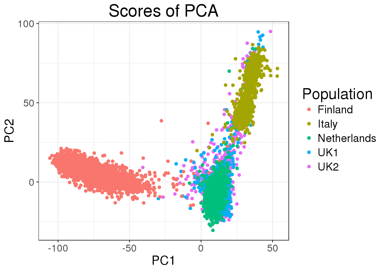
Suppose that we’ve obtained $n$ $p$-dimensional data points. For instance, let $n=100 000$ be the number of sequenced Russian citizen, and $n=300 000$ polymorphic single-nucleotide polymorphisms that characterize each Russian citizen. We want to clusterize the Russian population into sub-populations and visually inspect the results, by projecting each person from the initial 300,000-dimensional space onto a lower-dimensional space (2D or 3D).

For our 2D/3D representation, we want to select such axes, that preserve the most information about a person. To say it more formally, if we had one point, we want the distance from the real point to its projection onto our 2D/3D space to be minimal. Now that we have n points, we want the sum of squared distances from each of those points to its projection to be minimal.

E.g. if we chose to project the data onto a 2D-space, we are looking for such axes $v$ and $w$, that sum of square distances from points to their projections were minimal:

$v, w = \arg \min_{v, w} \sum \limits_{i=1}^{n} d^2(X_i, proj_{v,w} X_i)$

Minimal sum of square distance to the axes $\iff$ maximum explained variance

$proj^2_{v,w}X_i + d^2(X_i, proj_{v} X_i) = X_i^2$

$\sum \limits_{i=1}^{n} proj^2_{v,w}X_i + \sum \limits_{i=1}^{n} d^2(X_i, proj_{v} X_i) = \sum \limits_{i=1}^{n} X_i^2 = const$

$v, w = \arg \min_{v, w} \sum \limits_{i=1}^{n} d^2(X_i, proj_{v,w} X_i) = \arg \max_{v, w} \sum \limits_{i=1}^{n} proj_{v,w} X_i$

Thus, by choosing $v, w$ such, that they minimize the distances from the points to their projections, we simultaneously maximize the lengths of the projections themselves.

Iterative optimization process

Observation: turns out, you can use a greedy algorithm to perform the required optimization.

Indeed, if the dimensionality of space, that we are going to project the data to, is $m$, we can always choose an orthogonal basis in that m-dimensional subspace that we are looking for.

Thus, we can first find one axis $v$, such that:

$v = \arg \min_{v} \sum \limits_{i=1}^{n} d^2(X_i, proj_{v} X_i)$

Then we should find $w$, which is supposed to be orthogonal to $v$ so that:

$w = \arg \min_{w} \sum \limits_{i=1}^{n} d^2(X_i, proj_{w} X_i)$, and $w$ is orthogonal to $v$.

Next basis vector should be orthogonal to both $v$ and $w$, and so on. Luckily, as we’ll see in the next chapter, PCA automatically makes each next axis orthogonal to the previous ones.

Reformulation as an eigenvectors/eigenvalues problem

Alright, how do we find a single vector, such that projection onto it is maximal? Pretty simple, if the axis vector is $v$, the length of projection of $X_i$ data point onto it is $\frac{(v^T X_i)^2}{v^T v}$.

We are looking to maximize the sum of squares of lengths of the projections over all the data points:

$v = \arg \max_v \frac{v^T \bm{X}^T \bm{X} v}{v^T v} = \arg \max_v \frac{v^T \Sigma v}{v^T v}$, where $\Sigma = \frac{1}{n-1} \sum \limits_{i=1}^{n} (X_i - \hat{X})(X_i - \hat{X})^T$ is a sample covariance matrix.

By the way, the quantity $R(\Sigma, v) = \frac{v^T \Sigma v}{v^T v}$ is called Rayleigh quotient, as the covariance matrix is symmetric.

$\Sigma = E \Lambda E^T$, thus, $R(\Sigma, v) = \frac{(v^T E) \Lambda (E^T v)}{v^T v} = \frac{Y^T \Lambda Y}{v^T v}$, where $Y = E^T v$.

Elements of vector$Y$, $y_i$, are coefficients for i-th eigenvector; eigenvectors are orthogonal, because the covariance matrix is symmetric, thus $v^T v = v^T E E^T v = Y^T Y$.

Thus, $R(\Sigma, v) = R(\Sigma, Y) = \frac{Y^T \Lambda Y}{Y^T Y} = \frac{\sum \limits_{i=1}^{p} \lambda_i y_i^2}{ \sum \limits_{i=1}^{p} y_i^2 }$.

If one of the eigenvalues, say, $\lambda_q$, is larger than the others, as it often happens, it is called main eigenvalue.

The Rayleigh quotient then will take its maximal value, if $Y = (0, 0, ..., \underbrace{1}_\text{q-th position}, 0, ..., 0)^T$.

Indeed, let $z_i = y_i^2$, then we maximize the sum $\sum \limits_{i=1}^{p} \lambda_i z_i$ for non-negative $z_i$, given constraint $\sum \limits_{i=1}^{p} z_i = const$. Obviously, we reach maximum, if we maximize $z_q$, where $\lambda_q$ is the largest eigenvalue.

Classical statistics perspective

From multivariate normal distribution perspective.

TODO

SVD perspective

As was mentioned previously, PCA works with covariance matrix $\Sigma = X^T X$, where $X$ is our data vectors.

From the technical perspective, this matrix is as a special case of well-known in mathematics Gram matrix.

Gram matrices are positive semi-definite and symmetric. Moreover, usually they are non-full rank, if $X$ is $n$ x $p$ matrix, where $n > p$, which means that although $\Sigma$ has dimensionality $n \times n$, its rank is only $p$ and it has only $p$ non-zero eigenvalues.

Hence, a convenient technical way to find the eigenvalues of covariance matrix is Singular Value Decomposition:

$X = U D V^T$, where $U$ and $V$ are orthogonal $p \times p$ and $n \times n$ matrices, and $D$ is a diagonal $n \times p$ matrix of singular values (squares of singular values are eigenvalues of $\Sigma$), where only $p$ elements are non-zero.

For more details on SVD, read this post. For more details on properties of Gram matrix - read this one.

Stochastic processes and signal processing perspective

From the standpoint of Karhunen-Loeve theorem, PCA is similar to a Fourier series in digital signal processing - essentially, a way to perform a lossy compression.

We can interpret PCA as a decomposition of the input data matrix $X$ into an ordered series of matrices of rank 1, created by outer products of principal components. Let us re-write the SVD transform as a series of outer products:

$X = \sum \limits_{i=1}^{p} \lambda_i u_i v_i^T$, where $\lambda_i$ are eigenvalues, $u_i$ are column-vectors of matrix $U$ and $v_i^T$ are row-vectors of matrix $V^T$, so that $u_i v_i^T$ is an outer-product, resulting in a matrix of rank 1.

Each term of this sum contributes more to the resulting data matrix, the larger is the eigenvalue $\lambda_i$ in it. As in the case of Fourier transform, if we aim to compress the data, we can truncate the series early, when we believe that enough information is already contained in the first $x$ terms of the series. This approach is often used with SVD for data compression - e.g. eigenfaces approach, where whole datasets of human photos are compressed by early truncation of SVD series.

Bayesian optimization perspective

TODO: Vetrov’s lecture on VAE

References

• https://fmin.xyz/docs/applications/pca/ - source of cover image
• https://en.wikipedia.org/wiki/Karhunen%E2%80%93Lo%C3%A8ve_theorem
• https://en.wikipedia.org/wiki/Principal_component_analysis
• https://en.wikipedia.org/wiki/Rayleigh_quotient

Written by Boris Burkov who lives in Moscow, Russia, loves to take part in development of cutting-edge technologies, reflects on how the world works and admires the giants of the past. You can follow me in Telegram