


Goodness of fit tests - Kolmogorov-Smirnov, Cramer-von Mises, Anderson-Darling
October 01, 2026 36 min read
Previously we've already considered Chi-sqared goodness-of-fit (GoF) test in great detail. This post is dedicated to a different family of GoF tests, stemming from the same ideas of analysis of Brownian bridge, Karhunen-Loeve decomposition of infinite-dimentional covariance matrix of a stochastic process etc.
Goodness of Fit (GoF) problem
Goodness of fit problem arises when we need to check, if an empirically observed data follow some theoretically known distribution. E.g. we hypothesized that the distribution on the cover of this post is exponential. How to test, if this hypothesis holds?
Previously we’ve already considered derivation of Pearson’s Chi-squared goodness-of-fit test post.
Today we’ll look into a family of its alternatives, based on comparison of empirical distribution function with theoretical one. Then those tests would collect different statistics, all measuring some kind of divergence between theoretical and empirical distributions and will try to say that it is totally improbable to observe such an empirical distribution, if we assumed that indeed it was sampled from theoretical one.
Toolchain
All 3 tests, Kolmogorov-Smirnov, Cramer-von Mises, Anderson-Darling, rely upon the same set of mathematical objects and results. Hence, in order to understand the derivation of those tests and intuition behind them, I’ll first describe those objects and how they pertain to the GoF problem and then will consider specifics of each test in the final steps of their derivation, where they somewhat diverge (hopefully, this will result in intuitions on their relative advantages and disadvantages).
Empirical cumulative distribution function vs true distribution function
Let be i.i.d. with unknown CDF .
The empirical CDF is built out of samples from that distribution as the fraction of observations that have landed to the left of ,
.
The left subplot of the figure below is that for a standard Gaussian and samples; the blue curve is theoretical CDF , the red ladder is empirical CDF .
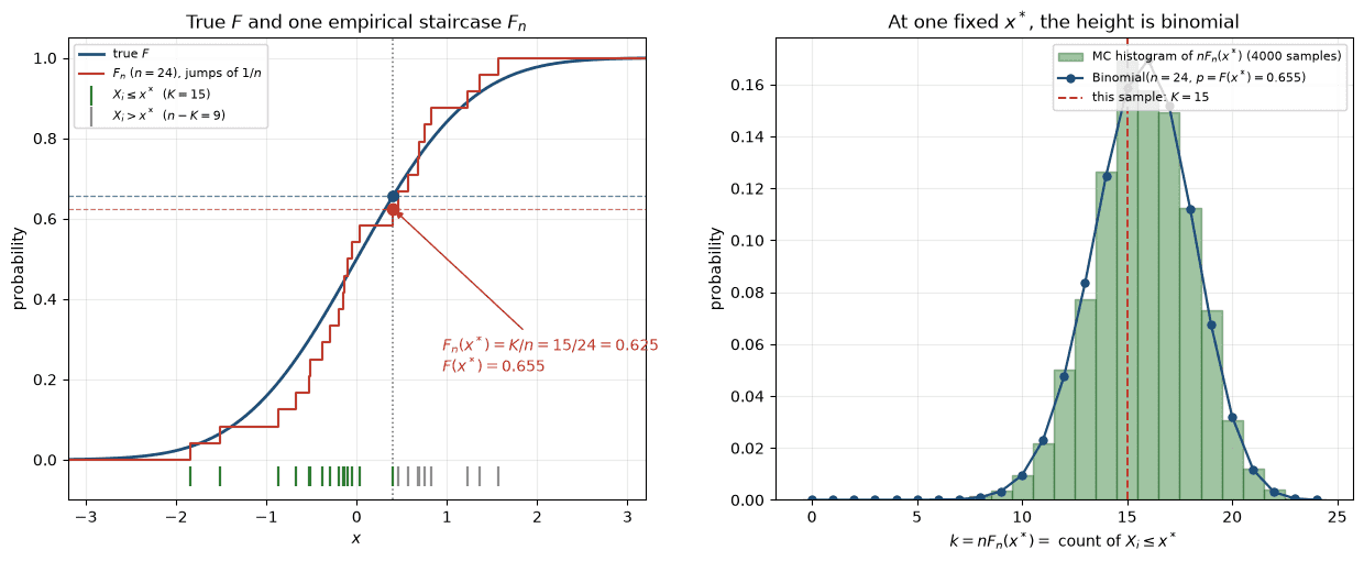
Now freeze a single abscissa (the dotted vertical line). The height no longer looks like a function — it is just a number , where counts how many green ticks sit to the left of . In the figure, out of , so , while the true height is .
Under the null hypothesis each independently falls on the left of with probability , so is a coin-flip count. That is why the histogram on the right is binomial, and why we next study pointwise before treating it as a process.
Binomial distribution of sample at each point
Now take a look at the right subplot of the figure above.
Fix a point on the real line and look at a single number: the height of the empirical CDF there, . Under the null, are i.i.d. from the hypothesized , so each indicator is a coin flip: . Hence , independent across . Their sum is binomial:
.
That is the whole story: “is the sample ?” is a yes/no trial with success probability , and we run independent trials. Immediately,
.
The variance is largest at the median () and vanishes in the tails — the empirical CDF is noisier in the middle than at the edges.
If the curve at the right reminds you a normal distribution, well, that’s because binomial distribution converges to normal in central part as : after centering and -scaling this binomial becomes approximately , which is exactly the pointwise marginal of the so-called Brownian bridge we will meet below.
Note however that this is a pointwise statement: the counts at two different and are dependent (the same sample is reused), so the process is not a collection of independent binomials.
Quantile transform
The binomial picture above still depends on : the success probability at is . Kolmogorov–Smirnov, Cramér–von Mises and Anderson–Darling get rid of that dependence with the quantile transform. If is continuous and , then
.
Proof is one line: for (for a general continuous CDF take the generalized inverse ).
So under the null, the mapped sample is i.i.d. uniform on . Write its empirical CDF as
.
The original ECDF is just this process reparametrized by the hypothesized CDF: . Comparing to is therefore the same as comparing to the identity map . In particular, from the previous section,
.
The whole GoF problem now lives on the unit interval, with a distribution-free null: no leftover . That is why the same critical values work for every continuous hypothesized law, and why the limiting object below is a Brownian bridge on rather than some -dependent process on .
If the null is false, is not uniform, drifts away from the diagonal, and that is what the tests detect. (If is estimated from the same sample, the are only approximately uniform — that is a different, composite, story.)
Brownian bridge
Pointwise, is a centered binomial, hence asymptotically .
GoF tests, however, are not questions about one : Kolmogorov–Smirnov looks at , Cramér–von Mises at , Anderson–Darling at a weighted version. Those are functionals of the whole path. Two hard constraints come with it: and always, so the centered process is pinned at both ends of . A Wiener process starts at but is free at . The Gaussian process that is Wiener-like and tied down at both endpoints is the Brownian bridge; Donsker’s theorem (next) says the empirical process converges to it.
Intuition: take a Wiener process (, independent Gaussian increments, ). It typically ends at some . Draw the chord from to and subtract it,
.
Then : the path is a “bridge” between the two banks of the interval. Equivalently, is Brownian motion conditioned on . That is the same geometry as the empirical process after the quantile transform: starts at (no mass before ) and returns to (all mass is accounted for by ). The figure below is exactly this construction.
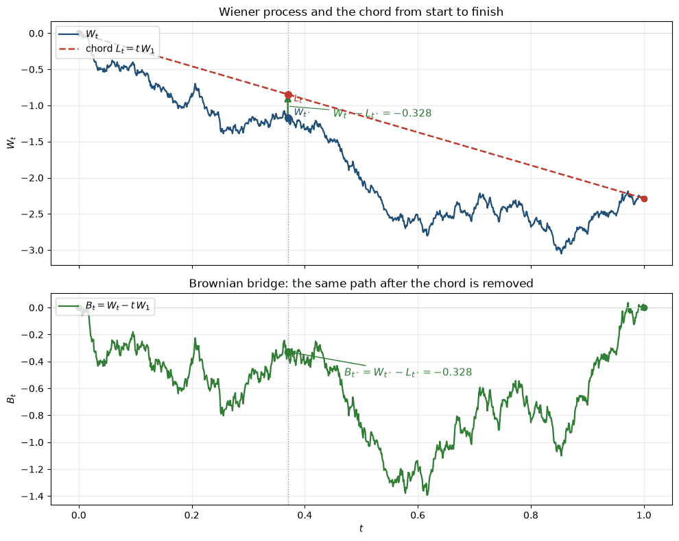
The object GoF actually computes with is this staircase, centered and blown up to CLT scale. Call it the empirical process
.
Pointwise it is the standardized binomial from earlier; as a function of it is a stochastic process that, like the green curve above, starts at and dies at . Without the , Glivenko–Cantelli says uniformly — the staircase hugs and there is nothing left to test. The keeps the typical fluctuations of order , so questions like “is too large?” have a non-degenerate answer. Donsker’s theorem, next, is the functional CLT that identifies the limiting path: , a Brownian bridge. That is the whole reason to care about bridges — every KS/CvM/AD statistic is a continuous functional of , hence in the limit a functional of , whose law we can actually compute.
Donsker’s theorem
Here the previous pieces become a theorem: we have an empirical staircase , a pinned fluctuation process , and a named Gaussian limit (Brownian bridge) that has the same covariance and the same endpoints. Donsker’s theorem is the statement that this is actually convergence in distribution: as stochastic processes on . The double arrow means convergence in distribution. In case of discrete random variable that is the statement at every continuity point of — equivalently, for every bounded continuous . In a continuous case of a stochastic process it is the same thing, with a bounded continuous functional of the whole curve: for every such . In particular it does not say that one realized staircase converges to one realized bridge ; only that probabilities of nice events about the path settle to those of .
That arrow is the hinge of the rest of the post. Write for a test statistic: a continuous map from a path on to a real number, (the arrow just names the function: “the path is sent to the number ”).
Kolmogorov–Smirnov, Cramér–von Mises and Anderson–Darling are three such maps:
The continuous mapping theorem plus Donsker turn into , whose laws we then compute (Kolmogorov’s distribution of ; Karhunen–Loève for the and weighted maps in case of Cramer - von Mises and Anderson - Darling). Without Donsker we would only have the pointwise binomial CLT from earlier — enough for one , useless for a supremum or an integral over all .
The classical CLT watches only the endpoint: . (A single arrow is the same idea as , but for a random number rather than a stochastic process.) Donsker’s theorem is the same statement for the whole path. We will prove two claims.
Donsker’s theorem (functional CLT).
Donsker’s theorem for the partial sums. Let be i.i.d. with mean and variance , , and on . Then , a standard Wiener process.
Donsker’s theorem for the empirical process. Let be i.i.d. Uniform and . Then , a standard Brownian bridge on . Equivalently is a Donsker walk with the chord subtracted: .
The first claim is steps 1–3; the second is step 4.
1. Rescale the walk. Let be i.i.d. with , , and (for the tightness step) a finite fourth moment. Put , , and
(linearly interpolate between if you prefer a continuous path). Time sits at ; height is the CLT scale . Ordinary CLT is .
2. Finite-dimensional distributions. Fix . The increments are functions of disjoint blocks of the , hence independent, and each block is a sum of about terms. Lindeberg CLT gives
,
independently across . Therefore converges to a centered Gaussian vector with — exactly the finite-dimensional laws of Wiener process .
3. Tightness (paths, not just coordinates). The finite-dimensional distributions (f.d.d.s) of a process are the laws of the random vectors for every finite grid . Step 2 says those vectors, for , converge to those of . That is not enough for as paths: two processes can agree on every finite grid and still differ wildly in the gaps (imagine a spike of height and width sitting between the ; no finite grid will see it, but will). Tightness rules those spikes out. A sequence of random paths is tight if, uniformly in , the path stays bounded and does not oscillate too fast: for every there is a modulus of continuity such that
is small, independently of . Then every subsequential limit is a continuous path, and together with the f.d.d.s it must be Wiener process.
The Kolmogorov–Chentsov theorem turns a moment bound on increments into that modulus. If a process satisfies, for some and ,
,
then it admits a version whose paths are almost surely Hölder- for every (locally: ). In particular the oscillations on small intervals are under control, which is tightness in Hölder geometry. For our walk the block of length and a finite fourth moment of give
,
which is Kolmogorov–Chentsov with , , hence Hölder up to (but not including) exponent — the same budget Brownian motion itself has (Wiener increments satisfy ). Tightness plus f.d.d.s as processes. (If you only assume two moments the same conclusion holds with a maximal inequality in place of Kolmogorov–Chentsov.)
4. Empirical process: the same two ingredients. After the quantile transform, . This is not a walk of independent increments in (each is reused), but it is a walk in the sample index, and the two Donsker steps still fire.
Finite-dimensional laws. For fixed , the vector of indicators is multinomial. We already computed its covariance: it equals at every finite . Multivariate CLT therefore sends to the corresponding Brownian-bridge vector. Also exactly.
Tightness. An increment is a centered binomial of success probability , hence the same fourth-moment bound . Tightness follows as in step 3.
The unique continuous Gaussian limit with that covariance and those endpoints is the Brownian bridge. Equivalently: the chord map is continuous, , and for a Donsker walk built from the same indicators, so continuous mapping gives directly from .
Continuous functionals of are then functionals of — which is how KS, CvM and AD get their null distributions.
Kolmogorov-Smirnov
The Kolmogorov–Smirnov statistic is the largest vertical gap between the staircase and the hypothesized CDF,
.
In the notation of the previous section this is just applied to the empirical process: . The supremum of a step function is attained at (or just before) a jump, so in practice one evaluates and at the order statistics and takes the max.
Donsker gives . The map is continuous, so the continuous mapping theorem yields the whole null distribution in one line:
.
The law of that supremum is Kolmogorov’s distribution. For ,
.
(The series is the reflection principle in disguise: is the probability that a bridge ever exits , obtained by summing signed Wiener paths that hit and still end at .) Thus, under a continuous simple null,
.
Reject when exceeds the -quantile of — about at , at . Because of the quantile transform, those numbers do not depend on .
KS asks only how far the worst point of wandered. That makes it a clean, distribution-free test of any continuous , and unusually sensitive to a single large bump. It is not equally sensitive everywhere: peaks at the median, so a deviation in the bulk moves more easily than the same vertical gap in the tails. Cramér–von Mises will average the squared gap instead of taking the max; Anderson–Darling will reweight the tails. If is estimated from the same sample, is no longer a free bridge and these critical values are too conservative (Lilliefors’ tables for normality, etc.).
Cramer-von Mises family of tests
Kolmogorov–Smirnov judged the empirical process by its size: one number, the worst vertical gap. The Cramér–von Mises family judges it in instead. Average the squared gap along the whole curve, optionally with a weight that says which you care about:
.
After the quantile transform this is the same as on the original scale. Two members of the family will occupy the rest of the post:
- Cramér–von Mises: , so ;
- Anderson–Darling: , so .
The AD weight is not a whim: , so puts the noisy middle and the quiet tails on equal footing. Both statistics are continuous maps of the path, so Donsker plus continuous mapping give under a continuous simple null — still distribution-free. What they share, and what KS did not need, is that the limit is a quadratic functional of a Gaussian process.
That is awkward at first glance. The random variables at different are dependent (the bridge covariance is not diagonal), so is not the square of one Gaussian and not an ordinary . The way out is the same move that turns a correlated Gaussian vector into independent coordinates: diagonalize , write with i.i.d. standard normal. For a process the covariance matrix is the kernel , the eigenvectors become eigenfunctions, and the finite sum becomes a series
That expansion is Karhunen–Loève — PCA in , with interdependent values of rotated into independent random coefficients in front of orthogonal eigenfunctions. Plug it into the quadratic statistic and the cross terms die:
,
a weighted sum of independent random variables. The eigenvalues depend on (plain for CvM, the inner product for AD), which is why the two tests get different series and different critical values — but they share this machinery. The next section builds that decomposition; then we return to the two choices of .
Karhunen-Loeve decomposition of a stochastic process
A finite-dimensional random vector is described by a covariance matrix . A standard way to diagonalize that covariance matrix is to perform a PCA or truncated PCA (knowing that the covariance matrix is Gram, i.e. symmetric positive definite, i.e. all of its eigenvalues are real and positive numbers and eigenvector correspond to the axes of ellipsoid of revolution). See post on PCA.
Karhunen-Loeve is a functional analysis-style generalization of PCA from discrete random vectors case to a continuous random function/stochastic process case. You can defined a covariance matrix for the stochastic process, describing how inter-correlated points of this process at a certain distance are.
In discrete case you sample a process at times and you get a random vector; let the grid get dense and you’re transitioning to a continuous random function case, where matrix becomes a covariance kernel . This is the same leap as from the discrete Fourier transform (eigenbasis of a circulant matrix on points) to Fourier series (eigenbasis of a translation-invariant kernel on ). In functional-analysis language, is a compact self-adjoint operator on , ; its eigen-decomposition is Karhunen–Loève — PCA for paths — which Cramér–von Mises and Anderson–Darling will use.
What’s counter-intuitive in this transition is that compared to discrete case axes change the roles: normally your data matrix would consist of data points, each of which is a -dimensional predictor. By covariance matrix you’d understand matrix of covariances between the data points, not between coordinates of each data point. Center the columns of (subtract each predictor’s mean) to get . The Gram matrix is the product of an matrix with a one, . Below , : the two blue rows of become the two blue columns of , and their inner product is the blue entry of .
In case of random functions and covariance kernel roles of axes swap. One path is what used to be a -dimensional data point, as . And so covariance kernel actually reflects correlations between what used to be your predictors. Flip the product: is times . The two orange columns of become the two orange rows of , and their inner product is the orange entry of the kernel — the object that becomes as .
(The usual sample-covariance or factor does not change the eigenstructure; it is omitted from the pictures.)
From practical standpoint for the Cramer - von Mises family of tests we’d need covariance kernels for Wiener process and for the Brownian bridge process . For the latter a short calculation gives
.
In particular . Not a coincidence: for ,
.
The empirical process on already has exactly the Brownian-bridge covariance at every finite (the multinomial structure of the indicators); only the marginals are still binomial rather than Gaussian. That is why this kernel is the right object: every path-functional of becomes, in the limit, the same functional of a Brownian bridge.
Cramer - von Mises
Cramér–von Mises is the unweighted member of the family, :
.
Every contributes equally to the energy of the empirical process. Relative to KS, a single spike is diluted by the rest of the curve; relative to AD, the tails are not up-weighted, so CvM is a bulk test — most of its power sits where is already large.
The staircase again turns the integral into a sum over :
.
(The term is the midpoint of the -th ECDF step; is the squared distance from the uniform order statistics to those midpoints, plus a continuity correction.)
Donsker sends to . Karhunen–Loève in ordinary diagonalizes the bridge covariance . The eigenfunctions and eigenvalues are the sine modes that vanish at both endpoints,
hence
This is a weighted generalized chi-squared with weights . The mode (a single arch on ) carries most of the mass; higher harmonics decay as , faster than AD’s , which is another way of saying CvM is less interested in the wiggly, tail-heavy part of the path.
Reject when is large. For a fully specified continuous the and points are about and $0.743.
Anderson–Darling, next, keeps this quadratic/KL story and only changes the inner product.
Anderson-Darling
Anderson–Darling is Cramér–von Mises with the weight that flattens the bridge’s variance, :
.
Near and , vanishes, so an ordinary gap (CvM) or a raw vertical gap (KS) can hide a large relative misfit in the tails. Dividing by is exactly studentizing each : the integrand is the square of the pointwise -score of . That is why AD is the member of the family people reach for when tail discrepancies matter (normality with outliers, exponential vs heavier tails, and so on).
Because is a staircase, the integral collapses to a sum over the order statistics of the quantile-transformed sample:
.
Under a continuous simple null, Donsker sends to . Karhunen–Loève in the weighted inner product diagonalizes that quadratic form. The eigenvalues of the corresponding operator on the bridge are , so
Each , so the limit is a weighted generalized chi-squared: an infinite linear combination of independent chi-squares, here with weights . It is “generalized” because it is not a single (the weights are unequal), and “weighted” because those are exactly the KL eigenvalues of the AD inner product. The same statement holds for CvM with a different sequence ; ordinary would require all weights equal.
(The eigenfunctions are Jacobi / shifted Legendre polynomials, orthonormal in that weighted — the same PCA story as CvM, different inner product, different spectrum. CvM’s eigenvalues decay like ; AD’s put relatively more mass on the first few modes.)
Reject when is large. For a fully specified continuous the and points of the limiting law are about and . As always, if mean or variance of is estimated from the same sample the process is no longer a free bridge and one must use the adjusted tables (Stephens); for normality that actually helps power, which is why AD is a standard normality test.
The three tests are now three functionals of the same : KS takes , CvM takes , AD takes . Same Donsker limit , three different ways of asking whether that bridge wandered too far.
Honorable mention: Shapiro-Wilk test of normality
Everything above was omnibus GoF: after the quantile transform, KS/CvM/AD do not care which continuous you hypothesized, and their null limits are functionals of one Brownian bridge. Shapiro–Wilk asks a narrower question — “is this sample Gaussian?” — and therefore throws away the empirical-process machinery. The mathematics is mostly different. The problem is the same, and the contrast is useful.
The catch we kept postponing is the composite null. In practice one almost never knows and ; one estimates them from the same sample. Then are not uniform, is not a free bridge, and the KS/CvM/AD critical values we quoted are wrong (Stephens / Lilliefors). Shapiro–Wilk is built for that case. It is location–scale invariant: , so unknown are not a nuisance — they are quotiented out.
The picture is a QQ-plot, which is the inverse of the ECDF story. Order the sample . Under normality the order statistics have known means and covariance for a standard normal sample . The best linear unbiased estimator of from those order statistics is (up to a constant). Shapiro–Wilk compares that Gaussian-specific estimate of scale to the ordinary sample variance:
; means the ordered sample lies exactly on the normal scores line. One rejects normality for small (the opposite direction from , , ). The Shapiro–Francia cousin is literally the squared correlation of with , i.e. of the QQ-plot; is that idea with the covariance of the order statistics baked into the weights .
So: KS/CvM/AD measure how far the ECDF staircase wanders from , in or (weighted) , and need Donsker to know what “far” means. Shapiro–Wilk measures how straight the quantile plot is against Gaussian order-statistic means, and “far” is a finite- ratio of quadratic forms — no bridge, no Karhunen–Loève, no generalized series. The payoff for specializing is power: for the composite normal null, typically beats even Anderson–Darling. The cost is that it does not test exponentiality, uniformity, or any other . Those remain jobs for .
References:

Written by Boris Burkov who lives in Moscow, Russia, loves to take part in development of cutting-edge technologies, reflects on how the world works and admires the giants of the past. You can follow me in Telegram